Year: 2024

Exploring causality with Python. Difference-in-differences

Establishing causality is one of modern analytics’s most essential and often neglected areas. I would like to describe and highlight the tools most used in our causal inference workshop in an upcoming series of articles.

Causal inference 101

Let’s start by defining causal inference. I will use Scott Cunningham’s definition from the Mixtape book.

He defines it as the study of estimating the impact of events and choices on a given outcome of interest. We are trying to establish the cause-and-effect relationship between variables (we can call them treatment and effect). It is a widespread problem in many areas, from business to public policy settings.

Usually, the setup of the causality-finding framework is relatively simple and consists of:

• treatment group — the group receiving the treatment
• control group — a group we want to treat as our benchmark to assess the treatment effect
• treatment — any activity directed to the treatment we wish to analyze
• outcome of interest

This setup is not just a theoretical concept, but a practical tool that can be applied to a wide range of real-world scenarios. From website optimization to A/B testing, from drug clinical trials to estimating the effect of development programs, the applications of causal inference are vast and diverse.

Let’s consider the conditions we must meet to establish a causal effect. First, we must assume that the treatment and control groups are comparable. Both should behave the same when treated and when untreated. For example, objects from the treatment group should behave the same as those from the control group had they not been treated.

And vice versa, objects from the control group should behave the same as those from the treatment group had they been treated. Hence, the only difference between those groups comes solely from the treatment. Comparing the outcome in the treatment group to the outcome in the control group gives us the treatment effect.

The control group is not just a comparison but a counterfactual for the treatment group. It shows us how the former would have behaved had it not been exposed to a given treatment. This underscores the crucial role of the control group in establishing causal effects.

The assumption that both groups are similar is strong and depends on the available data and research design. Achieving this comparability is the crucial task of causal inference.

Quasi — experiments

How can we obtain such conditions? Most articles tackling the topic of causality start with the notion that randomized experiments are the gold standard for establishing causality. However, they are often not feasible or practical to conduct.

Therefore, we are constantly looking for tools to help us find causal relationships. Research methods that tackle this problem are called quasi-experiments.

In the rest of the article, we will focus on one of the most important and often used quasi-experimental methods: difference-in-differences.

Minimum wage study

I will describe this method in the context of its classical application. To understand the approach, we will explore the work of Card and Kruger and their famous minimum wage study.

The effect of the minimum wage on employment is among the most heated debates in economics and public policy. The authors of the study tried to find an answer to this question. This type of problem is a perfect example of an issue we can’t explain using a randomized experiment. It would be practically impossible to randomly allocate certain groups or geographical regions to the different minimum wage levels.

In 1992, New Jersey increased the minimum wage from $4.25 to $5.05 per hour. Card and Kruger were looking for a benchmark against which to compare New Jersey.

Researchers decided to compare employment levels in New Jersey to those in Pennsylvania. The former state was chosen as the equivalent of a control group. They chose Pennsylvania because it is similar to New Jersey, both geographically and in terms of economic conditions.

They surveyed fast-food restaurants in both states before and after 1992 to check their number of employees. Scientists used employment in surveyed fast-food restaurants, as this business can quickly react to changes in the minimum wage.

Data set

Now’s the proper time to delve into the data. After the necessary data transformations (and simplifications for training purposes), we have the following data structure available. I used the data set from the David Card website (https://davidcard.berkeley.edu/data_sets.html):

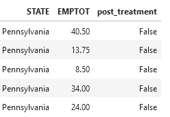
We can treat each row as the survey’s result in a restaurant. The crucial information is the state name, total employment, and the flag if the given record is from the period before or after the change in the minimum wage. We will treat the change in the minimum wage as a treatment variable in the analyzed study.

As a technical note, to make charting easier, we will store averages per time and state in a data frame:

An intuitive approach

How can we approach finding the effect of the minimum wage increase intuitively?

The most straightforward approach is to compare the average employment in both states after the treatment.

The chart shows that average employment in New Jersey was slightly lower than in Pennsylvania. Everyone who opposes the minimum wage is overjoyed and can conclude that this economic policy tool doesn’t work. Or is it perhaps too early to conclude?

Unfortunately, this approach is not correct. It omits crucial information about the pre-treatment differences in both states. The information we possess comes from something other than the randomized experiment, which makes it impossible to identify different factors that could account for the disparity between the two states.

These two states can be very different in terms of the number of people working there and the health of their economies. Comparing them after the treatment doesn’t reveal anything about the impact of the minimum wage and can result in inaccurate conclusions. I believe we should avoid this type of comparison in almost all cases.

Before/after comparison

We cannot draw conclusions based on comparing both states after the treatment. How about we look only at the state affected by the minimum wage change? Another way to evaluate the program’s impact is to compare employment in New Jersey before and after the change in the minimum wage. The chunk of code below does exactly this.

The before/after comparison presents a different picture. After raising the minimum wage, the average employment in fast-food restaurants in New Jersey increased.

Unfortunately, these conclusions are not definitive because this simple comparison has many flaws. The comparison between before and after the treatment makes one strong assumption: New Jersey’s employment level would have remained the same as before the change if the minimum wage had not increased.

Intuitively, it does not sound like a likely scenario. During this period, general economic activity had the potential to increase, government programs could have subsidized employment, and the restaurant industry could have experienced a significant surge in demand. Those are just some scenarios that could have influenced the employment level. It is typically not sufficient to establish the causal impact of the treatment by merely comparing the pre-and post-activity.

As a side note, this kind of comparison is quite common in various settings. Even though I think it’s more reliable than the previous approach we discussed, we should always be careful when comparing results.

Difference-in-differences

Finally, we have all the necessary elements in place to introduce the star of the show, a difference-in-differences method. We found that we can’t just compare two groups after the treatment to see if there is a causal effect. Comparing the treated group before and after treatment is also not enough. What about combining the two approaches?

Difference-in-differences analysis allows us to compare the changes in our outcome variable between selected groups over time. The time factor is crucial, as we can compare how something has changed since the treatment started. This approach’s simplicity is surprising, but like all causal approaches, it relies on assumptions.

We will cover different caveats later. Let’s start with the components needed to perform this evaluation exercise. DiD study requires at least two groups at two distinct times. One group is treated, and the other is used as a comparison group. We have to know at what point to compare groups. What items do we require for the task at hand?

• Pre-treatment value of the outcome variable from the control group
• Pre-treatment value of the outcome variable from the ‘treated’ group
• Post-treatment value of the outcome variable from the control group
• Post-treatment value of the outcome variable from the ‘treated’ group

As the next step, we have to compute the following metrics:

• The difference in outcome variables between the treated and control groups in the period before treatment.
• The difference in outcome variables between the treated and control groups after treatment.

And what are the next steps? We finally calculate the difference-in-differences, which is the difference between pre-treatment and post-treatment differences. This measure provides an estimate of the average treatment effect.

It’s easy to see the reasoning behind this strategy. The lack of data from the randomization experiment prevents us from comparing the differences between groups. However, it is possible to measure the difference between groups. A change in the difference in the outcome variable after treatment compared to the period before indicates a treatment effect.

Why is this? Before the treatment started, both groups had baseline values for the outcome variable. We assume that everything would have stayed the same in both groups if nothing had happened. However, the treatment occurred.

The treatment affected only one of the groups. Therefore, any changes in the outcome variable should only occur in the ‘treated’ group. Any change in the treatment group will change the outcome variable compared to the control group. This change is an effect of the treatment.

We assume the control group’s performance and trends will be the same as before treatment. Moreover, we must assume that the individuals in the treated group would have maintained their previous activity if the treatment had not occurred. The occurrence of treatment in one of the groups changes the picture and gives us the treatment effect.

Application

We can investigate the effect of minimum wage with our new tool by returning to our minimum wage example. With the information we have, we can figure out these numbers:

• Employment in New Jersey before the minimal wage increase
• Employment in Pennsylvania before the minimal wage increase
• Employment in New Jersey after the minimal wage increase
• Employment in Pennsylvania after the minimal wage increase

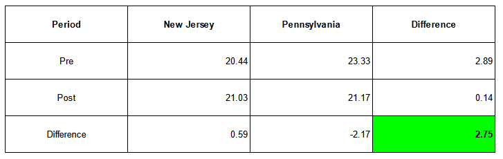
Before the minimum wage increased, Pennsylvania’s average employment in fast-food restaurants was higher. It changed after the increase, and the average employment difference between the two states was much smaller.

The code below calculates the differences between employment before and after the increase in the minimum wage (nj_difference and penn_difference). We also calculate the difference-in-difference estimate by subtracting both differences.

The code below plots differences to provide a nice visual comparison. Additionally, I am adding the counterfactual line. Technically, it is an estimate of the post-treatment employment in New Jersey if it had followed Pennsylvania’s trend. We will discuss this line in the next paragraph, which is crucial for understanding the difference-in-differences.

As you can see from the chart, the average employment in New Jersey increased by 0.59, while it decreased in Pennsylvania. Calculating the difference gives us an estimate of the treatment effect at 2.75. An increase in the minimum wage led to an increase in average employment, which is a surprising result.

Let us consider for a moment what caused these results. Employment in New Jersey did not increase significantly. However, the average employment rate in Pennsylvania decreased.

Without the minimum wage increase, we expect the average employment in New Jersey to follow the trend observed in Pennsylvania. If the minimum wage had not increased, average employment would have been lower.

On the chart, it is depicted as a counterfactual line, in which the New Jersey trend would follow the trend observed in Pennsylvania. The difference between the counterfactual line and the actual value observed in New Jersey equals the treatment effect of 2.75.

The introduction of the treatment changed this trend and allowed employment in New Jersey to maintain its value and slightly increase. What matters in this type of analysis is the change in magnitude of the treated group relative to the changes observed in the control group.

The table below summarizes the calculations in a format often encountered in DiD analysis. Treatment and control groups are represented in columns, the period in rows, and the measure of the outcome variable in cells.

The bottom-right corner displays the final estimate after calculating the differences.

Difference-in-differences using linear regression

I was writing about a simple calculation of a few averages. The difference-in-differences model’s computational simplicity is one of its advantages.

There are other ways to get those results. We could reach the same conclusions using a good, old linear regression. Expanding this model to multiple periods and groups would be beneficial.

One of the key advantages of the difference-in-differences model is its simplicity. We only need a handful of variables to run this model, making it straightforward and easy to use.

• Outcome variable: total employment (Y)
• Period: a dummy variable having a value of 0 before treatment and 1 in the treatment period (T)
• Group: a dummy variable having a value of 0 for a control group and 1 for a treatment group (G)

The model has the following form:

How can we interpret this model? B1 accounts for an increase in the value of the outcome variable when the treatment period starts. Our example shows the difference in the average employment in the control group after and before the treatment. We expect this change to happen without an increase in the minimum wage.

B2 accounts for a change in the outcome variable from the control to the treated group. It is the baseline difference between both groups — in a world before the treatment.

The interaction term (T*G) between the treatment period and the group shows the change in the outcome variable when both the treatment period and the treated group are activated. It has a value different from zero for a treated group in a treated period.

We want to achieve this in DiD analysis: the change of the outcome variable in the treated group during the treatment period compared to the control group.

There are many ways to calculate the results of this model in Python. For this example, we will use the statsmodels library. The specification of the linear model in our example looks like this:

As we can see in the regression output, the treatment effect (marked in yellow) is the same as calculated above. You can check that all the coefficients match the values calculated before.

It might seem like using regression analysis for simple average calculations is too much, but it has many benefits.

Firstly, the calculations are simpler than calculating averages for each group. We will also see the benefit of regression when we expand the model to include multiple comparison groups and periods.

What is also critical is that regression analysis allows us to assess the calculated parameters. We can obtain a confidence interval and p-value.

The results obtained by Card and Kruger were unexpected. They showed that an increase in the minimum wage does not negatively impact employment in the analyzed case. It even helped increase average employment.

This clever research indicates that we can find interesting and informative results even if we can’t do random experiments. It is the most fascinating aspect of causal inference that comes to mind when I think about it.

Main assumptions

Regression analysis concludes the application of the difference-in-differences model. This demonstration demonstrates how powerful this method can be. Before we finish, let’s think about the potential limitations of this model.

As for most of the causal inference, the model is as good as our assumptions about it. In this method, finding the correct group for comparison is crucial and requires domain expertise.

Whenever you read about difference-in-differences, you will encounter parallel trend assumptions. This signifies that before the treatment, both groups had a consistent trend in the outcome variable. The model also requires that those trends continue in the same direction over time and that the difference between both groups in the outcome variable stays the same in the absence of treatment.

In our example, we assume that average employment in fast-food restaurants in both states changes in the same way with time. If this assumption is not met, then the difference-in-difference analysis is biased.

History is one thing, but we also assume that this trend will continue over time, and this is something we will never know and cannot test.

This assumption is only partially testable. We can take a look at historical trends to assess if they are similar to each other. To achieve this, we need more historical data — even plotting the trends across times gives a good indicator of this assumption.

It is only partially testable, as we can only assess the behavior of the treated group if they had received treatment. We assume the affected group would have behaved the same as our control group, but we can’t be 100% certain. There is only one world we can assess. It is the fundamental problem of causal inference.

The difference-in-differences also requires the structure of both groups to remain the same over time. We need both groups to have the same composition before the treatment. They should have the same characteristics, except for their exposure to the treatment.

Summary

At first glance, all the assumptions might make this method less appealing. But is there any statistical or analytical approach without assumptions? We have to get as much quality data as possible, make sensitivity analyses, and use domain knowledge anyway. Then, we can find fascinating insights using differences-in-differences.

The post above has one disadvantage (and potentially many more — please let me know). It covers a relatively simple scenario — two groups and two periods. In the upcoming posts, I’ll further complicate this picture by employing the same technique but in a more complex setting.

I hope this explanation of the difference-in-differences method will help everyone who reads it. This article is my first step in sharing my learning with causal inference. More will follow.

References

Card, David & Krueger, Alan B, 1994. “Minimum Wages and Employment: A Case Study of the Fast-Food Industry in New Jersey and Pennsylvania,” American Economic Review, American Economic Association, vol. 84(4), pages 772–793, September

https://davidcard.berkeley.edu/data_sets.html

Impact Evaluation in Practice — Second Edition https://www.worldbank.org/en/programs/sief-trust-fund/publication/impact-evaluation-in-practice

https://mixtape.scunning.com/09-difference_in_differences

Exploring causality in Python. Difference-in-differences was originally published in Towards Data Science on Medium, where people are continuing the conversation by highlighting and responding to this story.