Holders, on average, had an unrealized profit of 4.5% on their initial investments.
PEPE looked bearish upon examination of its key technical indicators.
The rising digital economy is a largely unexplored territory with plenty of earning opportunities for everyone. However, a corporate-dominated sphere of influence uses complex tech terms to make it sound inaccessible to fun-loving, casual users. As a result, potential investors are left out, and digital coin collecting becomes an exclusive pastime for an unnecessary elite. […]
Pepecoin, known for its whimsical frog-themed design and devoted community, stands out amid a broader market recovery, where many cryptocurrencies are still struggling to regain their footing.
Bitcoin Ordinals explorer Ord.io has raised $2 million in a pre-seed funding round co-led by Bitcoin Frontier Fund and Sora Ventures to prepare for the highly anticipated launch of the Runes Protocol. Other investors in the round included Longhash Ventures, Daxos Capital, Portal Ventures, UTXO Management, Rubik Ventures, VitalTao Capital, Antalpha Ventures, Kommune Fund, Edessa […]
Marathon Digital executive claims BTC has already partially priced the halving.
Other execs disagree and expect BTC to follow previous cycles’ price action.
The DeFi sector in the blockchain industry is heating up with several narratives that have taken it by storm. Starting from artificial intelligence (AI) to web3 gaming, NFTs, and, more recently, real-world asset (RWA) platforms like ETFSwap (ETFS) spearheading the tokenization of assets. Tokenization is the new kid on the block, attracting institutional confidence as […]
Image by author and ChatGPT. “Design an illustration, featuring a Paralympic basketball player in action, this time the theme is on data pipelines” prompt. ChatGPT, 4, OpenAI, 15April. 2024. https://chat.openai.com.
In the previous post, we discussed how to use Notebooks with PySpark for feature engineering. While spark offers a lot of flexibility and power, it can be quite complex and requires a lot of code to get started. Not everyone is comfortable with writing code or has the time to learn a new programming language, which is where Dataflow Gen2 comes in.
What is Dataflow Gen2?
Dataflow Gen2 is a low-code data transformation and integration engine that allows you to create data pipelines for loading data from a wide variety of sources into Microsoft Fabric. It’s based on Power Query, which is integrated into many Microsoft products, such as Excel, Power BI, and Azure Data Factory. Dataflow Gen2 is a great tool for creating data pipelines without code via a visual interface, making it easy to create data pipelines quickly. If you are already familiar with Power Query or are not afraid of writing code, you can also use the underlying M (“Mashup”) language to create more complex transformations.
In this post, we will walk through how to use Dataflow Gen2 to create the same features needed to train our machine learning model. We will use the same dataset as in the previous post, which contains data about college basketball games.
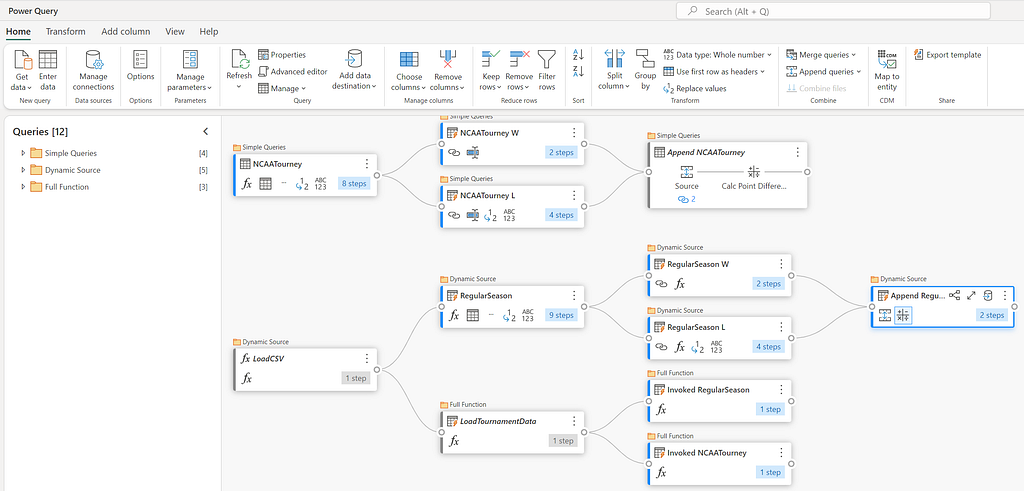
Fig. 1 — The final result. Image by author.
The Challenge
There are two datasets that we will be using to create our features: the regular season games and the tournament games. These two datasets are also split into the Men’s and Women’s tournaments, which will need to be combined into a single dataset. In total there are four csv files, that need to be combined and transformed into two separate tables in the Lakehouse.
Using Dataflows there are multiple ways to solve this problem, and in this post I want to show three different approaches: a no code approach, a low code approach and finally a more advanced all code approach.
The no code approach
The first and simplest approach is to use the Dataflow Gen2 visual interface to load the data and create the features.
The Data
The data we are looking at is from the 2024 US college basketball tournaments, which was obtained from the on-going March Machine Learning Mania 2024 Kaggle competition, the details of which can be found here, and is licensed under CC BY 4.0
Loading the data
The first step is to get the data from the Lakehouse, which can be done by selecting the “Get Data” button in the Home ribbon and then selecting More… from the list of data sources.
Fig. 2 — Choosing a data source. Image by author.
From the list, select OneLake data hub to find the Lakehouse and then once selected, find the csv file in the Files folder.
Fig. 3 — Select the csv file. Image by author.
This will create a new query with four steps, which are:
Source: A function that queries the Lakehouse for all the contents.
Navigation 1: Converts the contents of the Lakehouse into a table.
Navigation 2: Filters the table to retrieve the selected csv file by name.
Imported CSV: Converts the binary file into a table.
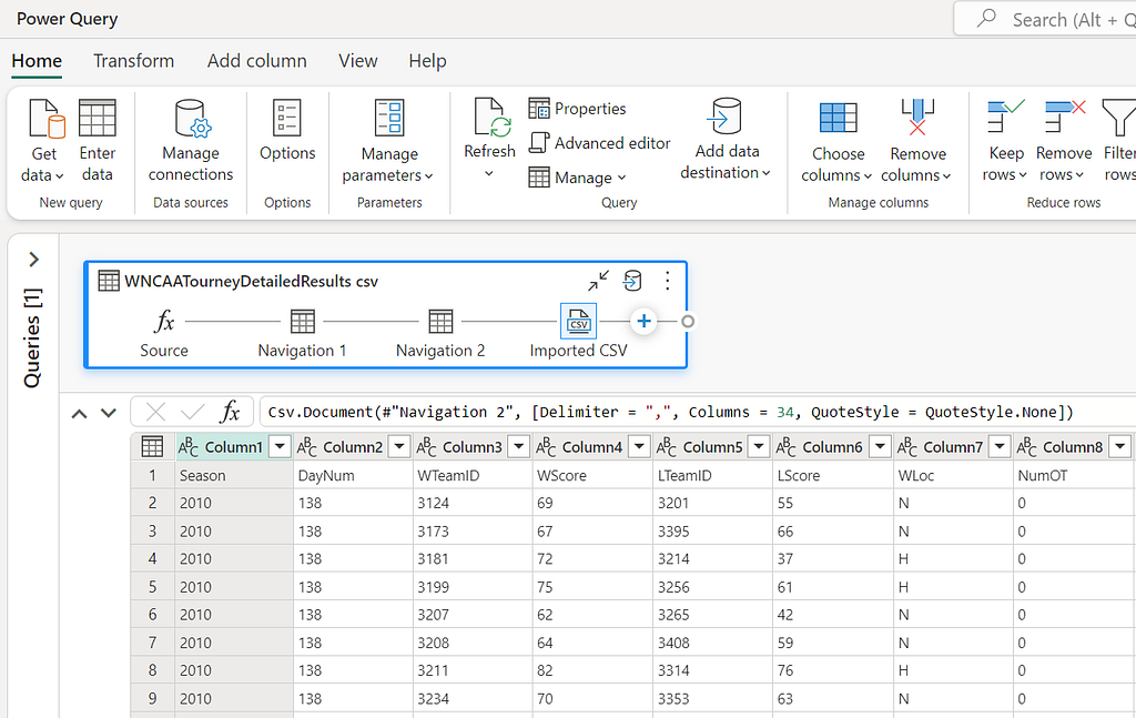
Fig. 4 — Initial load. Image by author.
Now that the data is loaded we can start with some basic data preparation to get it into a format that we can use to create our features. The first thing we need to do is set the column names to be based on the first row of the dataset. This can be done by selecting the “Use first row as headers” option in either the Transform group on the Home ribbon or in the Transform menu item.
The next step is to rename the column “WLoc” to “location” by either selecting the column in the table view, or by right clicking on the column and selecting “Rename”.
The location column contains the location of the game, which is either “H” for home, “A” for away, or “N” for neutral. For our purposes, we want to convert this to a numerical value, where “H” is 1, “A” is -1, and “N” is 0, as this will make it easier to use in our model. This can be done by selecting the column and then using the Replace values… transform in the Transform menu item.
Fig. 5 — Replace Values. Image by author.
This will need to be done for the other two location values as well.
Finally, we need to change the data type of the location column to be a Whole number instead of Text. This can be done by selecting the column and then selecting the data type from the drop down list in the Transform group on the Home ribbon.
Fig. 6 — Final data load. Image by author.
Instead of repeating the rename step for each of the location types, a little bit of M code can be used to replace the values in the location column. This can be done by selecting the previous transform in the query (Renamed columns) and then selecting the Insert step button in the formula bar. This will add a new step, and you can enter the following code to replace the values in the location column.
Table.ReplaceValue(#"Renamed columns", each [location], each if Text.Contains([location], "H") then "1" else if Text.Contains([location], "A") then "-1" else "0", Replacer.ReplaceText, {"location"})
Adding features
We’ve got the data loaded, but it’s still not right for our model. Each row in the dataset represents a game between two teams, and includes the scores and statistics for both the winning and losing team in a single wide table. We need to create features that represent the performance of each team in the game and to have a row per team per game.
To do this we need to split the data into two tables, one for the winning team and one for the losing team. The simplest way to do this is to create a new query for each team and then merge them back together at the end. There are a few ways that this could be done, however to keep things simple and understandable (especially if we ever need to come back to this later), we will create two references to the source query and then append them together again, after doing some light transformations.
Referencing a column can be done either from the Queries panel on the left, or by selecting the context menu of the query if using Diagram view. This will create a new query that references the original query, and any changes made to the original query will be reflected in the new query. I did this twice, once for the winning team and once for the losing team and then renamed the columns by prefixing them with “T1_” and “T2_” respectively.
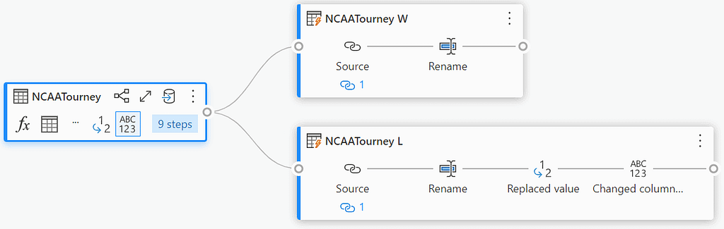
Fig. 7 — Split the dataset. Image by author.
Once the column values are set, we can then combine the two queries back together by using Append Queries and then create our first feature, which is the point difference between the two teams. This can be done by selecting the T1_Score and T2_Score columns and then selecting “Subtract” from the “Standard” group on the Add column ribbon.
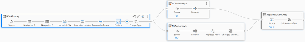
Now that’s done, we can then load the data into the Lakehouse as a new table. The final result should look something like this:
Fig. 8 — All joined up. Image by author.
There are a few limitations with the no code approach, the main one is that it’s not easy to reuse queries or transformations. In the above example we would need to repeat the same steps another three times to load each of the individual csv files. This is where copy / paste comes in handy, but it’s not ideal. Let’s look at a low code approach next.
The low code approach
In the low code approach we will use a combination of the visual interface and the M language to load and transform the data. This approach is more flexible than the no code approach, but still doesn’t require a lot of code to be written.
Loading the data
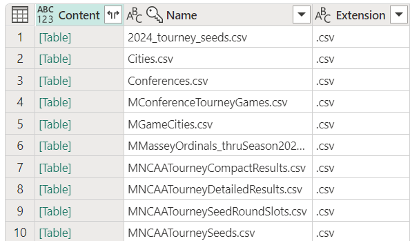
The goal of the low code approach is to reduce the number of repeated queries that are needed and to make it easier to reuse transformations. To do this we will take advantage of the fact that Power Query is a functional language and that we can create functions to encapsulate the transformations that we want to apply to the data. When we first loaded the data from the Lakehouse there were four steps that were created, the second step was to convert the contents of the Lakehouse into a table, with each row containing a reference to a binary csv file. We can use this as the input into a function, which will load the csv into a new table, using the Invoke custom function transformation for each row of the table.
Fig. 9 — Lakehouse query with the binary csv files in a column called Content. Image by author.
To create the function, select “Blank query” from the Get data menu, or right click the Queries panel and select “New query” > “Blank query”. In the new query window, enter the following code:
The code of this function has been copied from our initial no code approach, but instead of loading the csv file directly, it takes a parameter called TableContents, reads it as a csv file Csv.Document and then sets the first row of the data to be the column headers Table.PromoteHeaders.
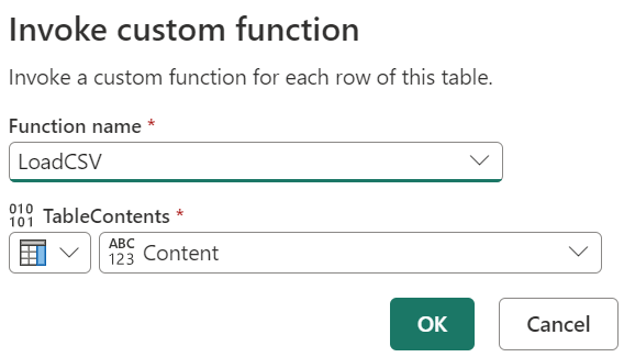
We can then use the Invoke custom function transformation to apply this function to each row of the Lakehouse query. This can be done by selecting the “Invoke custom function” transformation from the Add column ribbon and then selecting the function that we just created.
Fig. 10 — Invoke custom function. Image by author.
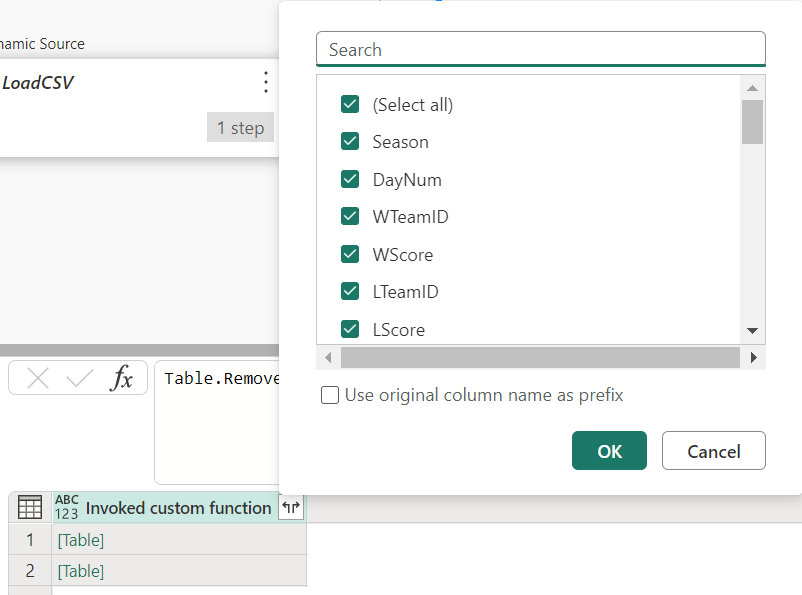
This will create a new column in the Lakehouse query, with the entire contents of the csv file loaded into a table, which is represented as [Table] in the table view. We can then use the expand function on the column heading to expand the table into individual columns.
Fig. 11 — Expand columns. Image by author.
The result effectively combines the two csv files into a single table, which we can then continue to create our features from as before.
There are still some limitations with this approach, while we’ve reduced the number of repeated queries, we still need to duplicate everything for both the regular season and tournament games datasets. This is where the all code approach comes in.
The all code approach
The all code approach is the most flexible and powerful approach, but also requires the most amount of code to be written. This approach is best suited for those who are comfortable with writing code and want to have full control over the transformations that are applied to the data.
Essentially what we’ll do is grab all the M code that was generated in each of the queries and combine them into a single query. This will allow us to load all the csv files in a single query and then apply the transformations to each of them in a single step. To get all the M code, we can select each query and then click on the Advanced Editor from the Home ribbon, which displays all the M code that was generated for that query. We can then copy and paste this code into a new query and then combine them all together.
To do this, we need to create a new blank query and then enter the following code:
Note: the Lakehouse connection values have been removed
What’s happening here is that we’re:
Loading the data from the Lakehouse;
Filtering the rows to only include the csv files that match the TourneyType parameter;
Loading the csv files into tables;
Expanding the tables into columns;
Renaming the columns;
Changing the data types;
Combining the two tables back together;
Calculating the point difference between the two teams.
Using the query is then as simple as selecting it, and then invoking the function with the TourneyType parameter.
Fig. 12 — Invoke function. Image by author.
This will create a new query with the function as it’s source, and the data loaded and transformed. It’s then just a case of loading the data into the Lakehouse as a new table.
Fig. 13 — Function load. Image by author.
As you can see, the LoadTournamentData function is invoked with the parameter “RegularSeasonDetailedResults” which will load both the Men’s and Women’s regular season games into a single table.
Conclusion
And that’s it!
Hopefully this post has given you a good overview of how to use Dataflow Gen2 to prepare data and create features for your machine learning model. Its low code approach makes it easy to create data pipelines quickly, and it contains a lot of powerful features that can be used to create complex transformations. It’s a great first port of call for anyone who needs to transform data, but more importantly, has the benefit of not needing to write complex code that is prone to errors, is hard to test, and is difficult to maintain.
At the time of writing, Dataflows Gen2 are unsupported with the Git integration, and so it’s not possible to version control or share the dataflows. This feature is expected to be released in Q4 2024.
Learn about the structure of LangChain pipelines, callbacks, how to create custom callbacks and integrate them into your pipelines for improved monitoring
Callbacks are an important functionality that helps with monitoring/debugging your pipelines. In this note, we cover the basics of callbacks and how to create custom ones for your use cases. More importantly, through examples, we also develop an understanding of the structure/componentization of LangChain pipelines and how that plays into the design of custom callbacks.
This note assumes basic familiarity with LangChain and how pipelines in LangChain work.
Basic Structure of Callbacks
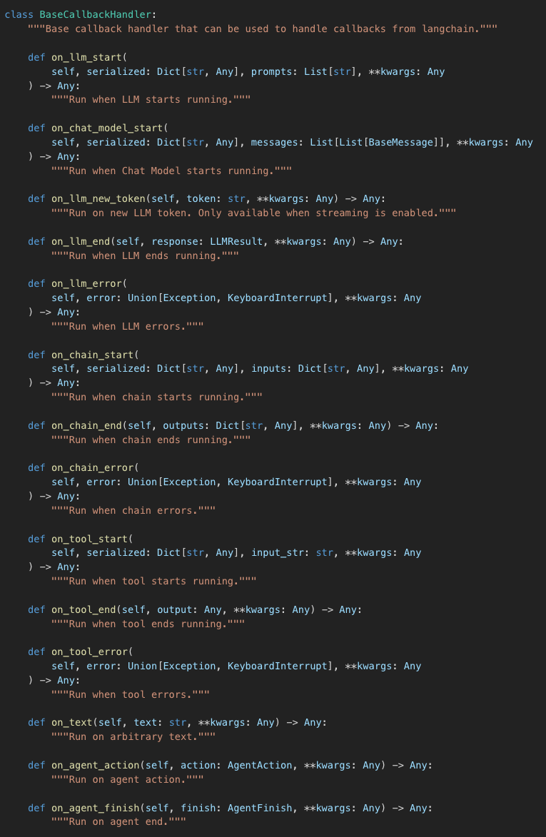
To learn about the basics of callbacks in LangChain, we start with the official documentation where we can find the definition of the BaseCallbackHandler class.
As you can see this is an abstract class that defines quite a few methods to cover various events in your LangChain pipeline. These methods can be grouped together into the following segments :
LLM [start, end, error, new token]
Chain [start, end, error]
Tool [start, end, error]
Agent [action, finish]
If you have worked with LangChain pipelines before, the methods along with their provided descriptions should be mostly self explanatory. For example, the on_llm_start callback is the event that gets triggered when the LangChain pipeline passes input to the LLM. And that on_llm_end is subsequently triggered when the LLM provides its final output.
NOTE : There are events triggers that can be used in addition to whats shown above. These can be found here. These cover triggers relating to Retrievers, Prompts, ChatModel etc.
Understanding how Callbacks work
Callbacks are a very common programming concept that have been widely used for a while now, so the high level concept of how callbacks work is well understood. So in this post, we focus on the specific nuances of how callbacks work in LangChain and how we could use it to satisfy our specific use cases.
Keeping in the mind the base Callback class that we saw in the previous section, we explore Callbacks in LangChain through a series of increasingly complex examples and in the process gain a better understanding of the structure of pipelines in LangChain. This would be a top-down approach to learning where we start with examples first and actual definitions later as I found that to be more useful personally for this specific topic.
Example 1
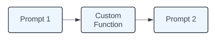
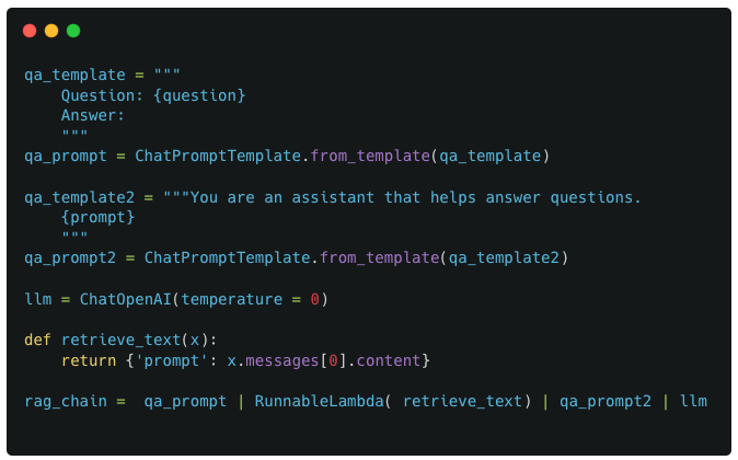
We start with a simple dummy chain that has 3 components : 2 prompts and a custom function to join them. I refer to this as a dummy example because its very unlikely that you would need two separate prompts to interact with each other, but it makes for an easier example to start with for understanding callbacks and LangChain pipelines.
Example 1 : Basic structure of LangChain pipeline
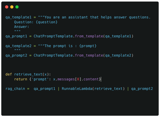
Implementing this in code would look like :
Pipeline implementation for Example 1
The above code is pretty textbook stuff. The only possibly complex piece is the retrieve_text and RunnableLambda function thats being used here. The reason this is necessary is because the format of the output from qa_prompt1 is not compatible with the format of the output required by qa_prompt2.
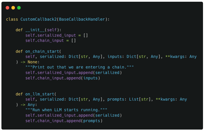
Defining the custom Callback
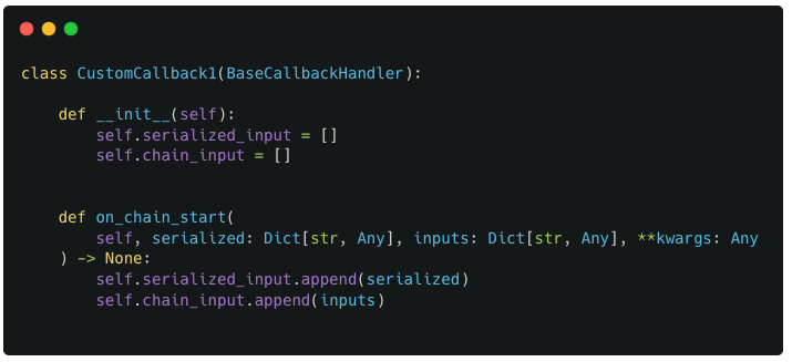
For our custom callback, we define a new subclass of BaseCallbackHandler called CustomCallback1 which defines the on_chain_start method. The method definition is straightforward as it simply takes the input values passed to it and saves it in 2 specific variables : chain_input and serialized_input
Invoking the custom callback
Example 1 : Invoking with pipeline with the custom callback
The above code shows one of the possible ways to pass your custom callback to your pipeline : As a list of callback objects as the value to a corresponding key of ‘callbacks’. This also makes it easy to guess that you can pass multiple callbacks to your LangChain pipeline.
Decoding the Callback/Pipeline Structure
Now comes the interesting part. After we have defined the callbacks and passed it on to our pipeline, we now perform a deep dive into the callback outputs
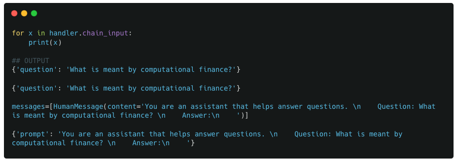
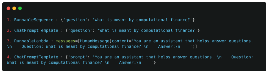
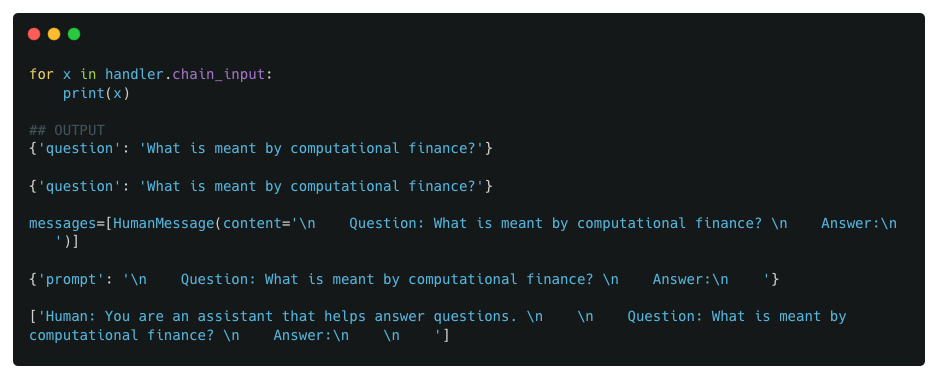
We first look at the values stored in chain_input
Example 1 : Contents of chain_input variable of callback handler
Observations :
Though there are 3 components in our chain, there are 4 values in chain_input. Which corresponds to the on_chain_start method being triggered 4 times instead of 3.
For the first two chain_input values/ on_chain_start triggers, the input is the same as the user provided input.
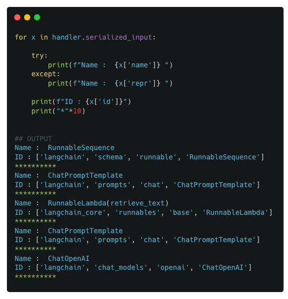
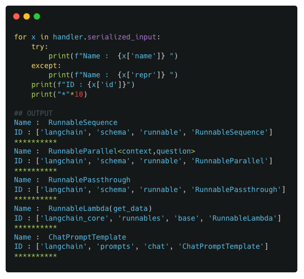
We next look at the outputs of serialized_input
Observations :
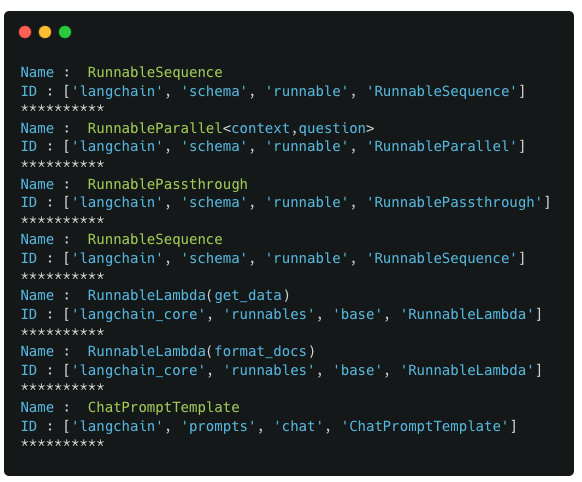
The first component is a RunnableSequence which is a component that wasnt added by the user but was automatically added by LangChain. The rest of the components correspond directly to the user-defined components in the pipeline.
The full contents of serialized_input is extensive! While there is a definite structure to that content, its definitely out of scope for this post and possibly doesnt have much practical implications for an end user.
How do we interpret these results
For the most part, the outputs seen in the chain_input and serialized_input make sense. Whether its the input values or the names/IDs of the components. The only largely unknown part is the RunnableSequence component, so we take a closer look at this.
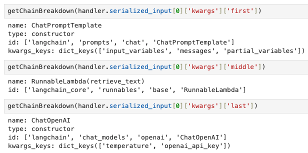
As I mentioned previously, the full contents of serialized_input is extensive and not easy to digest. So to make things easier, we look at only the high level attributes described in serialized_input and try to intrepret the results through these attributes. For this, we make use of a custom debugging function called getChainBreakdown (code in notebook).
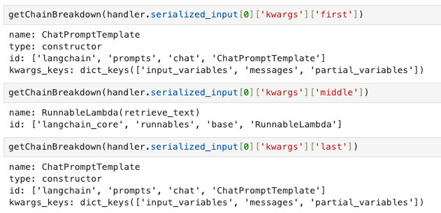
We call getChainBreakdown on all values of serialized_input and observe the output. Specifically for the first RunnableSequence element, we look at the keys of the kwargs dict : first, midde, last, name.
On closer inspection of the kwargs argument and their values, we see that they have the same structure as our previous pipeline components. In fact, the first, middle and last components correspond exactly to the user-defined components of the pipeline.
Closer inspection of RunnableSequence kwargs values
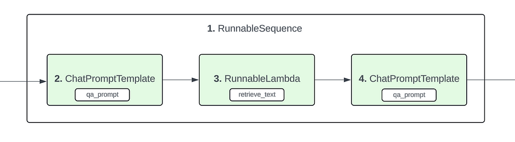
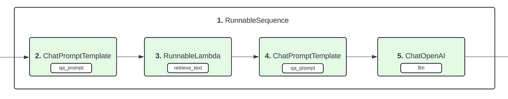
The above details form the basis of the final conclusion that we make here. That the structure of the pipeline is like shown below :
Example 1 : Structure of LangChain pipeline
We do make a bit of a leap here as the above flowchart was confirmed after going through a bunch of examples and observing the format in which these components are created internally by LangChain. So bear with me as we go through these other examples which will solidify the conclusion that we make here.
With the above defined structure, the other pieces of the puzzle fit together quite well. Focusing on the chain_input values, lets map them to the components (with their ordering) defined above.
Example 1 : Mapping chain_input values to pipeline components
Observations :
For RunnableSequence, as it acts like a wrapper for the whole pipeline, the input from the user acts as the input for the RunnableSequence component as well.
For the first ChatPromptTemplate (qa_prompt1), as the first ‘true’ component of the pipeline, it receives the direct input from the user
For RunnableLambda (retrieve_text), it receives as input the output from qa_prompt1, which is a Message object
For the last ChatPromptTemplate (qa_prompt2), it receives as input the output from retrieve_text, which is a dict with ‘prompt’ as its single key
The above breakdown shows how the structure of the pipeline described above fits perfectly with the data seen in serialized_input and chain_input
Example 2
For the next example, we extend Example 1 by adding a LLM as the final step.
Example 2 : Pipeline definition
For the callback, since we have now added a LLM into the mix, we define a new custom callback that additionally defines the on_llm_start method. It has the same functionality as on_chain_start where the input arguments are saved into the callback object variables : chain_input and serialized_input
Example 2 : New custom callback with added on_llm_start method
Proposing the Pipeline structure
At this stage, instead of evaluating the callback variables, we switch things up and propose the potential structure of the pipeline. Given what we had learnt from the first example, the following should be the potential structure of the pipeline
Example 2 : Proposed structure of pipeline
So we would have a RunnableSequence component as a wrapper for the pipeline. And additionally include a new ChatOpenAI object thats nested within the RunnableSequence component.
Validating proposed structure using data
We now look at the values of in the callback object to validate the above proposed structure.
We first look at the values stored in chain_input
Example 2 : chain_input values
And then the serialized_input values :
Example 2 : serialized_input values
As well as a deeper inspection of the RunnableSequence components
Example 2 : Closer inspection of RunnableSequence kwargs values
Observations :
The values of serialized_input validate the activation/trigger sequence that was proposed in the pipeline structure : RunnableSequence -> ChatPromptTemplate(qa_prompt1) -> RunnableLambda(retrieve_text) -> ChatPromptTemplate(qa_prompt2) -> ChatOpenAI
The values of chain_input also map correctly to the proposed structure. The only new addition is the fifth entry, which corresponds to the output from qa_prompt2, which is fed as input to the ChatOpenAI object
The components of the RunnableSequence kwargs also verify the proposed structure as the new ‘last’ element is the ChatOpenAI object
By this stage, you should have an intuitive understanding of how LangChain pipelines are structured and when/how different callback events are triggered.
Though we have only focused on Chain and LLM events so far, these translate well to the other Tool and Agent triggers as well
Example 3
For the next example, we progress to a more complex chain involving a parallel implementation (RunnableParallel)
Chain/Callback Implementation
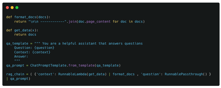
The chain has a parallel implementation as its first block which computes two values : context and question, which are then passed on to a prompt template to create the final prompt. The parallel functionality is required because we need to pass both context and question to the prompt template at the same time, where the context is retrived from a different source while the question is provided by the user.
For the context value, we use a static function get_data that returns the same piece of text (this is a dummy version of an actual retriever used in RAG applications).
Example 3 : Chain implementation
For the callback implementation, we use the same callback as the first example, CustomCallback1
Decoding the Callback/Pipeline Structure
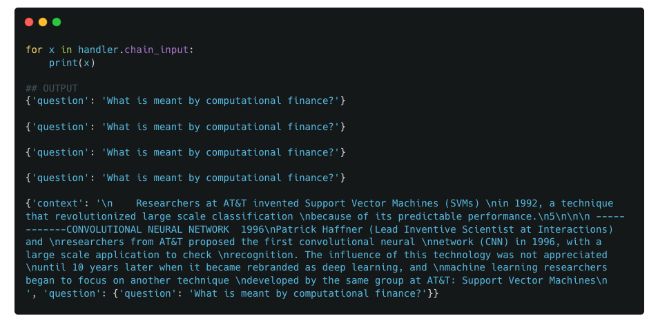
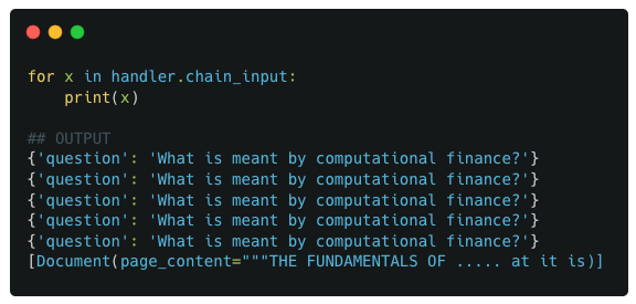
Similar to previous examples, we start by looking at the outputs of chain_input and serialized_input
Example 3 : chain_input valuesExample 3 : serialized_input values
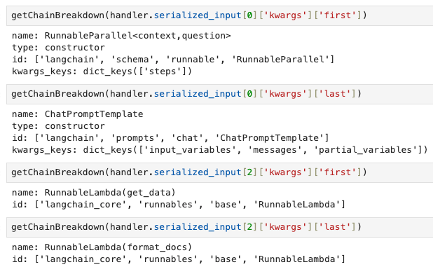
We also look do a deep dive into the RunnableSequence (index 0) and RunnableParallel (index 1) components
Observations :
Consistent with previous examples, the RunnableSequence acts as a wrapper to the whole pipeline. Its first component is the RunnableParallel component and its last component is the ChatPromptTemplate component
The RunnableParallel in turn encompasses two components : the RunnablePassthrough and the RunnableLambda (get_data).
The inputs to the first 4 components : RunnableSequence, RunnableParallel, RunnablePassthrough and RunnableLambda (get_data) are the same : the provided user input. Only for the final ChatPromptTemplate component do we have a different input, which is a dict with question and context keys.
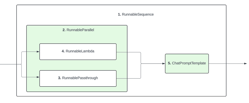
Based on these observations, we can infer the final structure of the pipeline as such :
Example 3 : Structure of LangChain pipeline
Example 4
Same as Example 3, but with an additional processing function for retrieving context
Chain/Callback Implementation
Example 4 : Chain implementation
Decoding the Callback/Pipeline Structure
Similar to previous examples, we again look at the usual data points
Example 4 : chain_input valuesExample 4 : serialized_input values
We observe that there are now 2 RunnableSequence components in our pipeline. So for the next step, we deep dive into both of these RunnableSequence components to see its internal components
Observations :
For the first RunnableSequence components, its components are the same as the previous example. Starts with RunnableParallel and ends with ChatPromptTemplate
For the second RunnableSequence, its first component is the RunnableLambda (get_data) component and the last component is the RunnableLambda (format_docs) component. This is basically the part of the pipeline responsible for generating the ‘context’ value. So its possible for a LangChain pipeline to have multiple RunnableSequence components to it. Especially when you are creating ‘sub-pipelines’
In this case, the creation of the ‘context’ value can be considered a pipeline by itself as it involves 2 different components chained together. So any such sub-pipelines in your primary pipeline will be wrapped up by a RunnableSequence component
3. The values from chain_input also match up well with the pipeline components and their ordering (Not going to breakdown each component’s input here as it should be self-explanatory by now)
So based on the above observations, the following is the identified structure of this pipeline
Example 4 : Structure of LangChain pipeline
Conclusion
The objective of this post was to help develop an (intuitive) understanding of how LangChain pipelines are structured and how callback triggers are associated with the pipeline.
By going through increasingly complex chain implementations, we were able to understand the general structure of LangChain pipelines and how a callback can be used for retrieving useful information. Developing an understanding of how LangChain pipelines are structured will also help facilitate the debugging process when errors are encountered.
A very common use case for callbacks is retrieving intermediate steps and through these examples we saw how we can implement custom callbacks that track the input at each stage of the pipeline. Add to this our understanding of the structure of the LangChain pipelines, we can now easily pinpoint the input to each component of the pipeline and retrieve it accordingly.
We use cookies on our website to give you the most relevant experience by remembering your preferences and repeat visits. By clicking “Accept”, you consent to the use of ALL the cookies.
This website uses cookies to improve your experience while you navigate through the website. Out of these, the cookies that are categorized as necessary are stored on your browser as they are essential for the working of basic functionalities of the website. We also use third-party cookies that help us analyze and understand how you use this website. These cookies will be stored in your browser only with your consent. You also have the option to opt-out of these cookies. But opting out of some of these cookies may affect your browsing experience.
Necessary cookies are absolutely essential for the website to function properly. These cookies ensure basic functionalities and security features of the website, anonymously.
Cookie
Duration
Description
cookielawinfo-checkbox-analytics
11 months
This cookie is set by GDPR Cookie Consent plugin. The cookie is used to store the user consent for the cookies in the category "Analytics".
cookielawinfo-checkbox-functional
11 months
The cookie is set by GDPR cookie consent to record the user consent for the cookies in the category "Functional".
cookielawinfo-checkbox-necessary
11 months
This cookie is set by GDPR Cookie Consent plugin. The cookies is used to store the user consent for the cookies in the category "Necessary".
cookielawinfo-checkbox-others
11 months
This cookie is set by GDPR Cookie Consent plugin. The cookie is used to store the user consent for the cookies in the category "Other.
cookielawinfo-checkbox-performance
11 months
This cookie is set by GDPR Cookie Consent plugin. The cookie is used to store the user consent for the cookies in the category "Performance".
viewed_cookie_policy
11 months
The cookie is set by the GDPR Cookie Consent plugin and is used to store whether or not user has consented to the use of cookies. It does not store any personal data.
Functional cookies help to perform certain functionalities like sharing the content of the website on social media platforms, collect feedbacks, and other third-party features.
Performance cookies are used to understand and analyze the key performance indexes of the website which helps in delivering a better user experience for the visitors.
Analytical cookies are used to understand how visitors interact with the website. These cookies help provide information on metrics the number of visitors, bounce rate, traffic source, etc.
Advertisement cookies are used to provide visitors with relevant ads and marketing campaigns. These cookies track visitors across websites and collect information to provide customized ads.