Year: 2024

Dive into the “Curse of Dimensionality” concept and understand the math behind all the surprising phenomena that arise in high dimensions.

In the realm of machine learning, handling high-dimensional vectors is not just common; it’s essential. This is illustrated by the architecture of popular models like Transformers. For instance, BERT uses 768-dimensional vectors to encode the tokens of the input sequences it processes and to better capture complex patterns in the data. Given that our brain struggles to visualize anything beyond 3 dimensions, the use of 768-dimensional vectors is quite mind-blowing!

While some Machine and Deep Learning models excel in these high-dimensional scenarios, they also present many challenges. In this article, we will explore the concept of the “curse of dimensionality”, explain some interesting phenomena associated with it, delve into the mathematics behind these phenomena, and discuss their general implications for your Machine Learning models.

Note that detailed mathematical proofs related to this article are available on my website as a supplementary extension to this article.

What is the curse of dimensionality?

People often assume that geometric concepts familiar in three dimensions behave similarly in higher-dimensional spaces. This is not the case. As dimension increases, many interesting and counterintuitive phenomena arise. The “Curse of Dimensionality” is a term invented by Richard Bellman (famous mathematician) that refers to all these surprising effects.

What is so special about high-dimension is how the “volume” of the space (we’ll explore that in more detail soon) is growing exponentially. Take a graduated line (in one dimension) from 1 to 10. There are 10 integers on this line. Extend that in 2 dimensions: it is now a square with 10 × 10 = 100 points with integer coordinates. Now consider “only” 80 dimensions: you would already have 10⁸⁰ points which is the number of atoms in the universe.

In other words, as the dimension increases, the volume of the space grows exponentially, resulting in data becoming increasingly sparse.

High-dimensional spaces are “empty”

Consider this other example. We want to calculate the farthest distance between two points in a unit hypercube (where each side has a length of 1):

• In 1 dimension (the hypercube is a line segment from 0 to 1), the maximum distance is simply 1.
• In 2 dimensions (the hypercube forms a square), the maximum distance is the distance between the opposite corners [0,0] and [1,1], which is √2, calculated using the Pythagorean theorem.
• Extending this concept to n dimensions, the distance between the points at [0,0,…,0] and [1,1,…,1] is √n. This formula arises because each additional dimension adds a square of 1 to the sum under the square root (again by the Pythagorean theorem).

Interestingly, as the number of dimensions n increases, the largest distance within the hypercube grows at an O(√n) rate. This phenomenon illustrates a diminishing returns effect, where increases in dimensional space lead to proportionally smaller gains in spatial distance. More details on this effect and its implications will be explored in the following sections of this article.

The notion of distance in high dimensions

Let’s dive deeper into the notion of distances we started exploring in the previous section.

We had our first glimpse of how high-dimensional spaces render the notion of distance almost meaningless. But what does this really mean, and can we mathematically visualize this phenomenon?

Let’s consider an experiment, using the same n-dimensional unit hypercube we defined before. First, we generate a dataset by randomly sampling many points in this cube: we effectively simulate a multivariate uniform distribution. Then, we sample another point (a “query” point) from that distribution and observe the distance from its nearest and farthest neighbor in our dataset.

Here is the corresponding Python code.

def generate_data(dimension, num_points):
    ''' Generate random data points within [0, 1] for each coordinate in the given dimension '''
    data = np.random.rand(num_points, dimension)
    return data


def neighbors(data, query_point):
    ''' Returns the nearest and farthest point in data from query_point '''
    nearest_distance = float('inf')
    farthest_distance = 0
    for point in data:
        distance = np.linalg.norm(point - query_point)
        if distance < nearest_distance:
            nearest_distance = distance
        if distance > farthest_distance:
            farthest_distance = distance
    return nearest_distance, farthest_distance

We can also plot these distances:

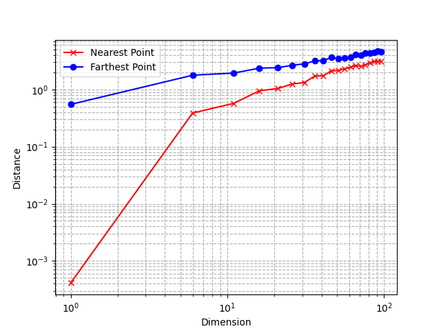
Using a log scale, we observe that the relative difference between the distance to the nearest and farthest neighbor tends to decrease as the dimension increases.

This is a very unintuitive behavior: as explained in the previous section, points are very sparse from each other because of the exponentially increasing volume of the space, but at the same time, the relative distances between points become smaller.

The notion of nearest neighbors vanishes

This means that the very concept of distance becomes less relevant and less discriminative as the dimension of the space increases. As you can imagine, it poses problems for Machine Learning algorithms that solely rely on distances such as kNN.

The maths: the n-ball

We will now talk about some other interesting phenomena. For this, we’ll need the n-ball. A n-ball is the generalization of a ball in n dimensions. The n-ball of radius R is the collection of points at a distance at most R from the center of the space 0.

Let’s consider a radius of 1. The 1-ball is the segment [-1, 1]. The 2-ball is the disk delimited by the unit circle, whose equation is x² + y² ≤ 1. The 3-ball (what we normally call a “ball”) has the equation x² + y² + z² ≤ 1. As you understand, we can extend that definition to any dimension:

The question now is: what is the volume of this ball? This is not an easy question and requires quite a lot of maths, which I won’t detail here. However, you can find all the details on my website, in my post about the volume of the n-ball.

After a lot of fun (integral calculus), you can prove that the volume of the n-ball can be expressed as follows, where Γ denotes the Gamma function.

For example, with R = 1 and n = 2, the volume is πR², because Γ(2) = 1. This is indeed the “volume” of the 2-ball (also called the “area” of a circle in this case).

However, beyond being an interesting mathematical challenge, the volume of the n-ball also has some very surprising properties.

As the dimension n increases, the volume of the n-ball converges to 0.

This is true for every radius, but let’s visualize this phenomenon with a few values of R.

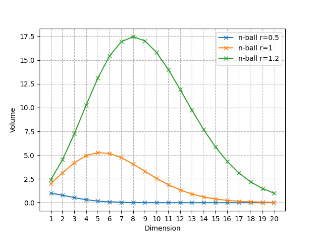
As you can see, it only converges to 0, but it starts by increasing and then decreases to 0. For R = 1, the ball with the largest volume is the 5-ball, and the value of n that reaches the maximum shifts to the right as R increases.

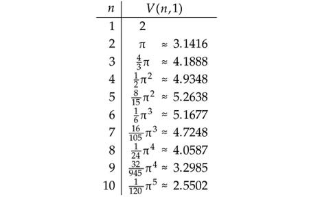
Here are the first values of the volume of the unit n-ball, up to n = 10.

The volume of a high-dimensional unit ball is concentrated near its surface.

For small dimensions, the volume of a ball looks quite “homogeneous”: this is not the case in high dimensions.

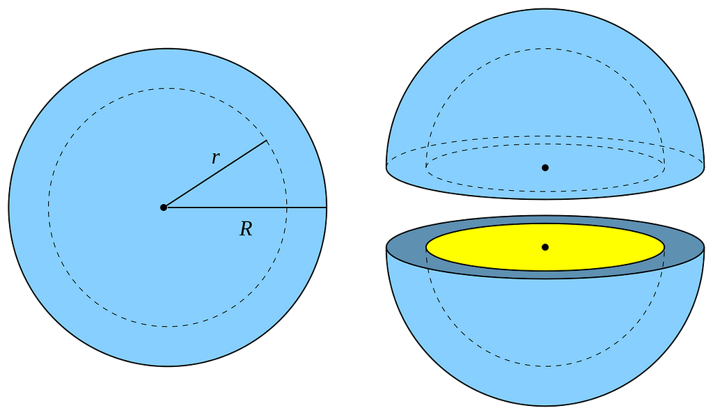
Let’s consider an n-ball with radius R and another with radius R-dR where dR is very small. The portion of the n-ball between these 2 balls is called a “shell” and corresponds to the portion of the ball near its surface(see the visualization above in 3D). We can compute the ratio of the volume of the entire ball and the volume of this thin shell only.

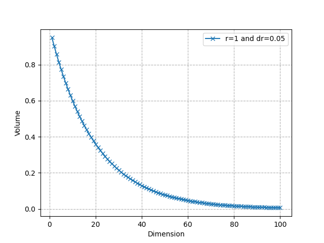
As we can see, it converges very quickly to 0: almost all the volume is near the surface in high dimensional spaces. For instance, for R = 1, dR = 0.05, and n = 50, about 92.3% of the volume is concentrated in the thin shell. This shows that in higher dimensions, the volume is in “corners”. This is again related to the distortion of the concept of distance we have seen earlier.

Note that the volume of the unit hypercube is 2ⁿ. The unit sphere is basically “empty” in very high dimensions, while the unit hypercube, in contrast, gets exponentially more points. Again, this shows how the idea of a “nearest neighbor” of a point loses its effectiveness because there is almost no point within a distance R of a query point q when n is large.

Curse of dimensionality, overfitting, and Occam’s Razor

The curse of dimensionality is closely related to the overfitting principle. Because of the exponential growth of the volume of the space with the dimension, we need very large datasets to adequately capture and model high-dimensional patterns. Even worse: we need a number of samples that grows exponentially with the dimension to overcome this limitation. This scenario, characterized by many features yet relatively few data points, is particularly prone to overfitting.

Occam’s Razor suggests that simpler models are generally better than complex ones because they are less likely to overfit. This principle is particularly relevant in high-dimensional contexts (where the curse of dimensionality plays a role) because it encourages the reduction of model complexity.

Applying Occam’s Razor principle in high-dimensional scenarios can mean reducing the dimensionality of the problem itself (via methods like PCA, feature selection, etc.), thereby mitigating some effects of the curse of dimensionality. Simplifying the model’s structure or the feature space helps in managing the sparse data distribution and in making distance metrics more meaningful again. For instance, dimensionality reduction is a very common preliminary step before applying the kNN algorithm. More recent methods, such as ANNs (Approximate Nearest Neighbors) also emerge as a way to deal with high-dimensional scenarios.

Blessing of dimensionality?

While we’ve outlined the challenges of high-dimensional settings in machine learning, there are also some advantages!

• High dimensions can enhance linear separability, making techniques like kernel methods more effective.
• Additionally, deep learning architectures are particularly adept at navigating and extracting complex patterns from high-dimensional spaces.

As always with Machine Learning, this is a trade-off: leveraging these advantages involves balancing the increased computational demands with potential gains in model performance.

Conclusion

Hopefully, this gives you an idea of how “weird” geometry can be in high-dimension and the many challenges it poses for machine learning model development. We saw how, in high-dimensional spaces, data is very sparse but also tends to be concentrated in the corners, and distances lose their usefulness. For a deeper dive into the n-ball and mathematical proofs, I encourage you to visit the extended of this article on my website.

While the “curse of dimensionality” outlines significant limitations in high-dimensional spaces, it’s exciting to see how modern deep learning models are increasingly adept at navigating these complexities. Consider the embedding models or the latest LLMs, for example, which utilize very high-dimensional vectors to more effectively discern and model textual patterns.

Want to learn more about Transformers and how they transform your data under the hood? Check out my previous article:

Transformers: How Do They Transform Your Data?

References:

• [1] “Volume of an n-ball.” Wikipedia, https://en.wikipedia.org/wiki/Volume_of_an_n-ball
• [2] “Curse of Dimensionality.” Wikipedia, https://en.wikipedia.org/wiki/Curse_of_dimensionality#Blessing_of_dimensionality
• [3] Peterson, Ivars. “An Adventure in the Nth Dimension.” American Scientist, https://www.americanscientist.org/article/an-adventure-in-the-nth-dimension
• [4] Zhang, Yuxi. “Curse of Dimensionality.” Geek Culture on Medium, July 2021, https://medium.com/geekculture/curse-of-dimensionality-e97ba916cb8f
• [5] “Approximate Nearest Neighbors (ANN).” Activeloop, https://www.activeloop.ai/resources/glossary/approximate-nearest-neighbors-ann/

The Math Behind “The Curse of Dimensionality” was originally published in Towards Data Science on Medium, where people are continuing the conversation by highlighting and responding to this story.

Learn how to reduce model latency when deploying Meta* Llama 3 on CPUs

The much-anticipated release of Meta’s third-generation batch of Llama is here, and I want to ensure you know how to deploy this state-of-the-art (SoTA) LLM optimally. In this tutorial, we will focus on performing weight-only-quantization (WOQ) to compress the 8B parameter model and improve inference latency, but first, let’s discuss Meta Llama 3.

Llama 3

To date, the Llama 3 family includes models ranging from 8B to 70B parameters, with more versions coming in the future. The models come with a permissive Meta Llama 3 license, you are encouraged to review before accepting the terms required to use them. This marks an exciting chapter for the Llama model family and open-source AI.

Architecture

The Llama 3 is an auto-regressive LLM based on a decoder-only transformer. Compared to Llama 2, the Meta team has made the following notable improvements:

• Adoption of grouped query attention (GQA), which improves inference efficiency.
• Optimized tokenizer with a vocabulary of 128K tokens designed to encode language more efficiently.
• Trained on a 15 trillion token dataset, this is 7x larger than Llama 2’s training dataset and includes 4x more code.

The figure below (Figure 1) is the result of print(model) where model is meta-llama/Meta-Llama-3–8B-Instruct. In this figure, we can see that the model comprises 32 LlamaDecoderLayers composed of Llama Attention self-attention components. Additionally, it has LlamaMLP, LlamaRMSNorm, and a Linear head. We hope to learn more once the Llama 3 research paper is released.

Language Modeling Performance

The model was evaluated on various industry-standard language modeling benchmarks, such as MMLU, GPQA, HumanEval, GSM-8K, MATH, and more. For the purpose of this tutorial, we will review the performance of the “Instruction Tuned Models” (Figure 2). The most remarkable aspect of these figures is that the Llama 3 8B parameter model outperforms Llama 2 70B by 62% to 143% across the reported benchmarks while being an 88% smaller model!

The increased language modeling performance, permissive licensing, and architectural efficiencies included with this latest Llama generation mark the beginning of a very exciting chapter in the generative AI space. Let’s explore how we can optimize inference on CPUs for scalable, low-latency deployments of Llama 3.

Optimizing Llama 3 Inference with PyTorch

In a previous article, I covered the importance of model compression and overall inference optimization in developing LLM-based applications. In this tutorial, we will focus on applying weight-only quantization (WOQ) to meta-llama/Meta-Llama-3–8B-Instruct. WOQ offers a balance between performance, latency, and accuracy, with options to quantize to int4 or int8. A key component of WOQ is the dequantization step, which converts int4/in8 weights back to bf16 before computation.

Environment Setup

You will need approximately 60GB of RAM to perform WOQ on Llama-3-8B-Instruct. This includes ~30GB to load the full model and ~30GB for peak memory during quantization. The WOQ Llama 3 will only consume ~10GB of RAM, meaning we can free ~50GB of RAM by releasing the full model from memory.

You can run this tutorial on the Intel® Tiber® Developer Cloud free JupyterLab* environment. This environment offers a 4th Generation Intel® Xeon® CPU with 224 threads and 504 GB of memory, more than enough to run this code.

If running this in your own IDE, you may need to address additional dependencies like installing Jupyter and/or configuring a conda/python environment. Before getting started, ensure that you have the following dependencies installed.

intel-extension-for-pytorch==2.2
transformers==4.35.2
torch==2.2.0
huggingface_hub

Accessing and Configuring Llama 3

You will need a Hugging Face* account to access Llama 3’s model and tokenizer.

To do so, select “Access Tokens” from your settings menu (Figure 4) and create a token.

Copy your access token and paste it into the “Token” field generated inside your Jupyter cell after running the following code.

from huggingface_hub import notebook_login, Repository

# Login to Hugging Face
notebook_login()

Go to meta-llama/Meta-Llama-3–8B-Instruct and carefully evaluate the terms and license before providing your information and submitting the Llama 3 access request. Accepting the model’s terms and providing your information is yours and yours alone.

Quantizing Llama-3–8B-Instruct with WOQ

We will leverage the Intel® Extension for PyTorch* to apply WOQ to Llama 3. This extension contains the latest PyTorch optimizations for Intel hardware. Follow these steps to quantize and perform inference with an optimized Llama 3 model:

1. Llama 3 Model and Tokenizer: Import the required packages and use the AutoModelForCausalLM.from_pretrained() and AutoTokenizer.from_pretrained() methods to load the Llama-3–8B-Instruct specific weights and tokenizer.

import torch
import intel_extension_for_pytorch as ipex
from transformers import AutoTokenizer, AutoModelForCausalLM, TextStreamer

Model = 'meta-llama/Meta-Llama-3-8B-Instruct'

model = AutoModelForCausalLM.from_pretrained(Model)
tokenizer = AutoTokenizer.from_pretrained(Model)

2. Quantization Recipe Config: Configure the WOQ quantization recipe. We can set the weight_dtype variable to the desired in-memory datatypes, choosing from torch.quint4x2 or torch.qint8 for int4 and in8, respectively. Additionally we can use lowp_model to define the dequantization precision. For now, we will keep this as ipex.quantization.WoqLowpMode.None to keep the default bf16 computation precision.

qconfig = ipex.quantization.get_weight_only_quant_qconfig_mapping(
  weight_dtype=torch.quint4x2, # or torch.qint8
  lowp_mode=ipex.quantization.WoqLowpMode.NONE, # or FP16, BF16, INT8
)
checkpoint = None # optionally load int4 or int8 checkpoint

# PART 3: Model optimization and quantization
model_ipex = ipex.llm.optimize(model, quantization_config=qconfig, low_precision_checkpoint=checkpoint)

del model 

We use ipex.llm.optimize() to apply WOQ and then del model to delete the full model from memory and free ~30GB of RAM.

3. Prompting Llama 3: Llama 3, like LLama 2, has a pre-defined prompting template for its instruction-tuned models. Using this template, developers can define specific model behavior instructions and provide user prompts and conversation history.

system= """nn You are a helpful, respectful and honest assistant. Always answer as helpfully as possible, while being safe. If you don't know the answer to a question, please don't share false information."""
user= "nn You are an expert in astronomy. Can you tell me 5 fun facts about the universe?"
model_answer_1 = 'None'

llama_prompt_tempate = f"""
<|begin_of_text|>n<|start_header_id|>system<|end_header_id|>{system}
<|eot_id|>n<|start_header_id|>user<|end_header_id|>{user}
<|eot_id|>n<|start_header_id|>assistant<|end_header_id|>{model_answer_1}<|eot_id|>
"""

inputs = tokenizer(llama_prompt_tempate, return_tensors="pt").input_ids

We provide the required fields and then use the tokenizer to convert the entire template into tokens for the model.

4. Llama 3 Inference: For text generation, we leverage TextStreamer to generate a real-time inference stream instead of printing the entire output at once. This results in a more natural text generation experience for readers. We provide the configured streamer to model_ipex.generate() and other text-generation parameters.

with torch.inference_mode():
    tokens = model_ipex.generate(
        inputs,
        streamer=streamer,
        pad_token_id=128001,
        eos_token_id=128001,
        max_new_tokens=300,
        repetition_penalty=1.5,
)

Upon running this code, the model will start generating outputs. Keep in mind that these are unfiltered and non-guarded outputs. For real-world use cases, you will need to make additional post-processing considerations.

That’s it. With less than 20 lines of code, you now have a low-latency CPU optimized version of the latest SoTA LLM in the ecosystem.

Considerations for Deployment

Depending on your inference service deployment strategy, there are a few things that you will want to consider:

• If deploying instances of Llama 3 in containers, WOQ will offer a smaller memory footprint and allow you to serve multiple inference services of the model on a single hardware node.
• When deploying multiple inference services, you should optimize the threads and memory reserved for each service instance. Leave enough additional memory (~4 GB) and threads (~4 threads) to handle background processes.
• Consider saving the WOQ version of the model and storing it in a model registry to eliminate the need to re-quantize the model per instance deployment.

Conclusion and Discussion

Meta’s Llama 3 LLM family delivers remarkable improvements over previous generations with a diverse range of configurations (8B to 70B). In this tutorial, we explored enhancing CPU inference with weight-only quantization (WOQ), a technique that minimizes latency while preserving accuracy.

By integrating the new generation of performance-oriented Llama 3 LLMs with optimization techniques like WOQ, developers can unlock new possibilities for GenAI applications. This combination simplifies the hardware requirements to achieve high-fidelity, low-latency results from LLMs integrated into new and existing systems.

A few exciting things to try next would be:

1. Experiment with Quantization Levels: You should test int4 and int8 quantization to identify the best compromise between performance and accuracy for your specific applications.
2. Performance Monitoring: It is crucial to continuously assess the performance and accuracy of the Llama 3 model across different real-world scenarios to ensure that quantization maintains the desired effectiveness.
3. Test more Llamas: Explore the entire Llama 3 family and evaluate the impact of WOQ and other PyTorch quantization recipes.

Thank you for reading! Don’t forget to follow my profile for more articles like this!

*Other names and brands may be claimed as the property of others.

Meta Llama 3 Optimized CPU Inference with Hugging Face and PyTorch was originally published in Towards Data Science on Medium, where people are continuing the conversation by highlighting and responding to this story.