Experts predict SOL could hit $501.78 by December 2024, ETH may surge to $7,280.98 soon, and Milei Moneda’s (MEDA) presale attracts significant investor interest. #partnercontent
The SEC is suing a Bitcoin mining company Geosyn, alleging that the firm engaged in an unregistered securities offering, raising over $5.6 million through deceptive practices. The U.S. Securities and Exchange Commission (SEC) has filed a lawsuit against Geosyn Mining,…
Enhanced relation extraction by fine-tuning Llama3–8B with a synthetic dataset created using Llama3–70B
Generated with DALL-E.
Premise
Relation extraction (RE) is the task of extracting relationships from unstructured text to identify connections between various named entities. It is done in conjunction with named entity recognition (NER) and is an essential step in a natural langage processing pipeline. With the rise of Large Language Models (LLMs), traditional supervised approaches that involve tagging entity spans and classifying relationships (if any) between them are enhanced or entirely replaced by LLM-based approaches [1].
Llama3 is the most recent major release in the domain of GenerativeAI [2]. The base model is available in two sizes, 8B and 70B, with a 400B model expected to be released soon. These models are available on the HuggingFace platform; see [3] for details. The 70B variant powers Meta’s new chat website Meta.ai and exhibits performance comparable to ChatGPT. The 8B model is among the most performant in its class. The architecture of Llama3 is similar to that of Llama2, with the increase in performance primarily due to data upgrading. The model comes with an upgaded tokenizer and expanded context window. It is labelled as open-source, although only a small percentage of the data is released. Overall, it is an excellent model, and I cannot wait to give it a try.
Llama3–70B can produce amazing results, but due to its size it is impractical, prohibitively expensive and hard to use on local systems. Therefore, to leverage its capabilities, we have Llama3–70B teach the smaller Llama3–8B the task of relation extraction from unstructured text.
Specifically, with the help of Llama3–70B, we build a supervised fine-tuning dataset aimed at relation extraction. We then use this dataset to fine-tune Llama3–8B to enhance its relation extraction capabilities.
To reproduce the code in the Google Colab Notebook associated to this blog, you will need:
HuggingFace credentials (to save the fine-tuned model, optional) and Llama3 access, which can be obtained by following the instructions from one of the models’ cards;
A free GroqCloud account (you can loggin with a Google account) and a corresponding API Key.
Workspace Setup
For this project I used a Google Colab Pro equipped with an A100 GPU and a High-RAM setting.
We start by installing all the required libraries:
I was very pleased to notice that the entire setup worked from the beginning without any dependencies issues or the need to install transformers from the source, despite the novelty of the model.
We also need to give access Goggle Colab to the drive and files and set the working directory:
# For Google Colab settings
from google.colab import userdata, drive

# This will prompt for authorization
drive.mount('/content/drive')

# Set the working directory
%cd '/content/drive/MyDrive/postedBlogs/llama3RE'
For those who wish to upload the model to the HuggingFace Hub, we need to upload the Hub credentials. In my case, these are stored in Google Colab secrets, which can be accessed via the key button on the left. This step is optional.
# For Hugging Face Hub setting
from huggingface_hub import login

# Upload the HuggingFace token (should have WRITE access) from Colab secrets
HF = userdata.get('HF')

# This is needed to upload the model to HuggingFace
login(token=HF,add_to_git_credential=True)
I also added some path variables to simplify file access:
# Create a path variable for the data folder
data_path = '/content/drive/MyDrive/postedBlogs/llama3RE/datas/'

# Full fine-tuning dataset
sft_dataset_file = f'{data_path}sft_train_data.json'

# Data collected from the the mini-test
mini_data_path = f'{data_path}mini_data.json'

# Test data containing all three outputs
all_tests_data = f'{data_path}all_tests.json'

# The adjusted training dataset
train_data_path = f'{data_path}sft_train_data.json'

# Create a path variable for the SFT model to be saved locally
sft_model_path = '/content/drive/MyDrive/llama3RE/Llama3_RE/'
Now that our workspace is set up, we can move to the first step, which is to build a synthetic dataset for the task of relation extraction.
Creating a Synthetic Dataset for Relation Extraction with Llama3–70B
There are several relation extraction datasets available, with the best-known being the CoNLL04 dataset. Additionally, there are excellent datasets such as web_nlg, available on HuggingFace, and SciREX developed by AllenAI. However, most of these datasets come with restrictive licenses.
Inspired by the format of the web_nlg dataset we will build our own dataset. This approach will be particularly useful if we plan to fine-tune a model trained on our dataset. To start, we need a collection of short sentences for our relation extraction task. We can compile this corpus in various ways.
Gather a Collection of Sentences
We will use databricks-dolly-15k, an open source dataset generated by Databricks employees in 2023. This dataset is designed for supervised fine-tuning and includes four features: instruction, context, response and category. After analyzing the eight categories, I decided to retain the first sentence of the context from the information_extraction category. The data parsing steps are outlined below:
from datasets import load_dataset

# Load the dataset
dataset = load_dataset("databricks/databricks-dolly-15k")

# Choose the desired category from the dataset
ie_category = [e for e in dataset["train"] if e["category"]=="information_extraction"]

# Retain only the context from each instance
ie_context = [e["context"] for e in ie_category]

# Split the text into sentences (at the period) and keep the first sentence
reduced_context = [text.split('.')[0] + '.' for text in ie_context]

# Retain sequences of specified lengths only (use character length)
sampler = [e for e in reduced_context if 30 < len(e) < 170]
The selection process yields a dataset comprising 1,041 sentences. Given that this is a mini-project, I did not handpick the sentences, and as a result, some samples may not be ideally suited for our task. In a project designated for production, I would carefully select only the most appropriate sentences. However, for the purposes of this project, this dataset will suffice.
Format the Data
We first need to create a system message that will define the input prompt and instruct the model on how to generate the answers:
system_message = """You are an experienced annontator.
Extract all entities and the relations between them from the following text.
Write the answer as a triple entity1|relationship|entitity2.
Do not add anything else.
Example Text: Alice is from France.
Answer: Alice|is from|France.
"""
Since this is an experimental phase, I am keeping the demands on the model to a minimum. I did test several other prompts, including some that requested outputs in CoNLL format where entities are categorized, and the model performed quite well. However, for simplicity’s sake, we’ll stick to the basics for now.
We also need to convert the data into a conversational format:
messages = [[
    {"role": "system","content": f"{system_message}"},
    {"role": "user", "content": e}] for e in sampler]
The Groq Client and API
Llama3 was released just a few days ago, and the availability of API options is still limited. While a chat interface is available for Llama3–70B, this project requires an API that could process my 1,000 sentences with a couple lines of code. I found this excellent YouTube video that explains how to use the GroqCloud API for free. For more details please refer to the video.
Just a reminder: you’ll need to log in and retrieve a free API Key from the GroqCloud website. My API key is already saved in the Google Colab secrets. We start by initializing the Groq client:
import os
from groq import Groq

gclient = Groq(
    api_key=userdata.get("GROQ"),
)
Next we need to define a couple of helper functions that will enable us to interact with the Meta.ai chat interface effectively (these are adapted from the YouTube video):
import time
from tqdm import tqdm

def process_data(prompt):

    """Send one request and retrieve model's generation."""

    chat_completion = gclient.chat.completions.create(
        messages=prompt, # input prompt to send to the model
        model="llama3-70b-8192", # according to GroqCloud labeling
        temperature=0.5, # controls diversity
        max_tokens=128, # max number tokens to generate
        top_p=1, # proportion of likelihood weighted options to consider
        stop=None, # string that signals to stop generating
        stream=False, # if set partial messages are sent
    )
    return chat_completion.choices[0].message.content


def send_messages(messages):

    """Process messages in batches with a pause between batches."""

   batch_size = 10
    answers = []

    for i in tqdm(range(0, len(messages), batch_size)): # batches of size 10

        batch = messages[i:i+10]  # get the next batch of messages

        for message in batch:
            output = process_data(message)
            answers.append(output)

        if i + 10 < len(messages):  # check if there are batches left
            time.sleep(10)  # wait for 10 seconds

    return answers
The first function process_data() serves as a wrapper for the chat completion function of the Groq client. The second function send_messages(), processes the data in small batches. If you follow the Settings link on the Groq playground page, you will find a link to Limits which details the conditions under which we can use the free API, including caps on the number of requests and generated tokens. To avoid exceedind these limits, I added a 10-seconds delay after each batch of 10 messages, although it wasn’t strictly necessary in my case. You might want to experiment with these settings.
What remains now is to generate our relation extraction data and integrate it with the initial dataset :
# Data generation with Llama3-70B
answers = send_messages(messages)

# Combine input data with the generated dataset
combined_dataset = [{'text': user, 'gold_re': output} for user, output in zip(sampler, answers)]
Evaluating Llama3–8B for Relation Extraction
Before proceeding with fine-tuning the model, it’s important to evaluate its performance on several samples to determine if fine-tuning is indeed necessary.
Building a Testing Dataset
We will select 20 samples from the dataset we just constructed and set them aside for testing. The remainder of the dataset will be used for fine-tuning.
import random
random.seed(17)

# Select 20 random entries
mini_data = random.sample(combined_dataset, 20)

# Build conversational format
parsed_mini_data = [[{'role': 'system', 'content': system_message},
                     {'role': 'user', 'content': e['text']}] for e in mini_data]

# Create the training set
train_data = [item for item in combined_dataset if item not in mini_data]
We will use the GroqCloud API and the utilities defined above, specifying model=llama3-8b-8192 while the rest of the function remains unchanged. In this case, we can directly process our small dataset without concern of exceeded the API limits.
Here is a sample output that provides the original text, the Llama3-70B generation denoted gold_re and the Llama3-8B hgeneration labelled test_re.
{'text': 'Long before any knowledge of electricity existed, people were aware of shocks from electric fish.',
 'gold_re': 'people|were aware of|shocksnshocks|from|electric fishnelectric fish|had|electricity',
 'test_re': 'electric fish|were aware of|shocks'}
Just from this example, it becomes clear that Llama3–8B could benefit from some improvements in its relation extraction capabilities. Let’s work on enhancing that.
Supervised Fine Tuning of Llama3–8B
We will utilize a full arsenal of techniques to assist us, including QLoRA and Flash Attention. I won’t delve into the specifics of choosing hyperparameters here, but if you’re interested in exploring further, check out these great references [4] and [5].
The A100 GPU supports Flash Attention and bfloat16, and it possesses about 40GB of memory, which is sufficient for our fine-tuning needs.
Preparing the SFT Dataset
We start by parsing the dataset into a conversational format, including a system message, input text and the desired answer, which we derive from the Llama3–70B generation. We then save it as a HuggingFace dataset:
from transformers import AutoModelForCausalLM
from peft import prepare_model_for_kbit_training
from trl import setup_chat_format

device_map = {"": torch.cuda.current_device()} if torch.cuda.is_available() else None

model = AutoModelForCausalLM.from_pretrained(
    model_id,
    device_map=device_map,
    attn_implementation="flash_attention_2",
    quantization_config=bnb_config
)

model, tokenizer = setup_chat_format(model, tokenizer)
model = prepare_model_for_kbit_training(model)
LoRA Configuration
from peft import LoraConfig

# According to Sebastian Raschka findings
peft_config = LoraConfig(
        lora_alpha=128, #32
        lora_dropout=0.05,
        r=256,  #16
        bias="none",
        target_modules=["q_proj", "o_proj", "gate_proj", "up_proj",
          "down_proj", "k_proj", "v_proj"],
        task_type="CAUSAL_LM",
)
The best results are achieved when targeting all the linear layers. If memory constraints are a concern, opting for more standard values such as alpha=32 and rank=16 can be beneficial, as these settings result in significantly fewer parameters.
Training Arguments
from transformers import TrainingArguments

# Adapted from  Phil Schmid blogpost
args = TrainingArguments(
    output_dir=sft_model_path,              # directory to save the model and repository id
    num_train_epochs=2,                     # number of training epochs
    per_device_train_batch_size=4,          # batch size per device during training
    gradient_accumulation_steps=2,          # number of steps before performing a backward/update pass
    gradient_checkpointing=True,            # use gradient checkpointing to save memory, use in distributed training
    optim="adamw_8bit",                     # choose paged_adamw_8bit if not enough memory
    logging_steps=10,                       # log every 10 steps
    save_strategy="epoch",                  # save checkpoint every epoch
    learning_rate=2e-4,                     # learning rate, based on QLoRA paper
    bf16=True,                              # use bfloat16 precision
    tf32=True,                              # use tf32 precision
    max_grad_norm=0.3,                      # max gradient norm based on QLoRA paper
    warmup_ratio=0.03,                      # warmup ratio based on QLoRA paper
    lr_scheduler_type="constant",           # use constant learning rate scheduler
    push_to_hub=True,                       # push model to Hugging Face hub
    hub_model_id="llama3-8b-sft-qlora-re",
    report_to="tensorboard",               # report metrics to tensorboard
    )
If you choose to save the model locally, you can omit the last three parameters. You may also need to adjust the per_device_batch_size and gradient_accumulation_steps to prevent Out of Memory (OOM) errors.
Initialize the Trainer and Train the Model
from trl import SFTTrainer

trainer = SFTTrainer(
    model=model,
    args=args,
    train_dataset=sft_dataset,
    peft_config=peft_config,
    max_seq_length=512,
    tokenizer=tokenizer,
    packing=False, # True if the dataset is large
    dataset_kwargs={
        "add_special_tokens": False,  # the template adds the special tokens
        "append_concat_token": False, # no need to add additional separator token
    }
)

trainer.train()
trainer.save_model()
The training, including model saving, took about 10 minutes.
Let’s clear the memory to prepare for inference tests. If you’re using a GPU with less memory and encounter CUDA Out of Memory (OOM) errors, you might need to restart the runtime.
import torch
import gc
del model
del tokenizer
gc.collect()
torch.cuda.empty_cache()
Inference with SFT Model
In this final step we will load the base model in half precision along with the Peft adapter. For this test, I have chosen not to merge the model with the adapter.
from peft import AutoPeftModelForCausalLM
from transformers import AutoTokenizer, pipeline
import torch

# HF model
peft_model_id = "solanaO/llama3-8b-sft-qlora-re"

# Load Model with PEFT adapter
model = AutoPeftModelForCausalLM.from_pretrained(
  peft_model_id,
  device_map="auto",
  torch_dtype=torch.float16,
  offload_buffers=True
)
We load the test dataset, which consists of the 20 samples we set aside previously, and format the data in a conversational style. However, this time we omit the assistant message and format it as a Hugging Face dataset:
Question: Long before any knowledge of electricity existed, people were aware of shocks from electric fish.

Gold-RE: people|were aware of|shocks
    shocks|from|electric fish
    electric fish|had|electricity

LLama3-8B-RE: electric fish|were aware of|shocks

SFT-Llama3-8B-RE: people|were aware of|shocks
         shocks|from|electric fish
In this example, we observe significant improvements in the relation extraction capabilities of Llama3–8B through fine-tuning. Despite the fine-tuning dataset being neither very clean nor particularly large, the results are impressive.
For the complete results on the 20-sample dataset, please refer to the Google Colab notebook. Note that the inference test takes longer because we load the model in half-precision.
Conclusion
In conclusion, by utilizing Llama3–70B and an available dataset, we successfully created a synthetic dataset which was then used to fine-tune Llama3–8B for a specific task. This process not only familiarized us with Llama3, but also allowed us to apply straightforward techniques from Hugging Face. We observed that working with Llama3 closely resembles the experience with Llama2, with the notable improvements being enhanced output quality and a more effective tokenizer.
For those interested in pushing the boundaries further, consider challenging the model with more complex tasks such as categorizing entities and relationships, and using these classifications to build a knowledge graph.
References
Somin Wadhwa, Silvio Amir, Byron C. Wallace, Revisiting Relation Extraction in the era of Large Language Models, arXiv.2305.05003 (2023).
Meta, Introducing Meta Llama 3: The most capable openly available LLM to date, April 18, 2024 (link).
Welcome to my series on Causal AI, where we will explore the integration of causal reasoning into machine learning models. Expect to explore a number of practical applications across different business contexts.
In the last article we explored de-biasing treatment effects with Double Machine Learning. This time we will delve further into the potential of DML covering using Double Machine Learning and Linear Programming to optimise treatment strategies.
If you missed the last article on Double Machine Learning, check it out here:
This article will showcase how Double Machine Learning and Linear Programming can be used optimise treatment strategies:
Expect to gain a broad understanding of:
Why businesses want to optimise treatment strategies.
How conditional average treatment effects (CATE) can help personalise treatment strategies (also known as Uplift modelling).
How Linear Programming can be used to optimise treatment assignment given budget constraints.
A worked case study in Python illustrating how we can use Double Machine Learning to estimate CATE and Linear Programming to optimise treatment strategies.
There is a common question which arises in most businesses: “What is the optimal treatment for a customer in order to maximise future sales whilst minimising cost?”.
Let’s break this idea down with a simple example.
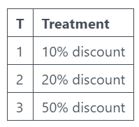
Your business sells socks online. You don’t sell an essential product, so you need to encourage existing customers to repeat purchase. Your main lever for this is sending out discounts. So the treatment strategy in this case is sending out discounts:
10% discount
20% discount
50% discount
Each discount has a different return on investment. If you think back to the last article on average treatment effects, you can probably see how we can calculate ATE for each of these discounts and then select the one with the highest return.
However, what if we have heterogenous treatment effects — The treatment effect varies across different subgroups of the population.
This is when we need to start considering conditional average treatment effects (CATE)!
Conditional Average Treatment Effects (CATE)
CATE
CATE is the average impact of a treatment or intervention on different subgroups of a population. ATE was very much about “does this treatment work?” whereas CATE allows us to change the question to “who should we treat?”.
We “condition” on our control features to allow treatment effects to vary depending on customer characteristics.
Think back to the example where we are sending out discounts. If customers with a higher number of previous orders respond better to discounts, we can condition on this customer characteristic.
It is worth pointing out that in Marketing, estimating CATE is often referred to as Uplift Modelling.
Estimating CATE with Double Machine Learning
We covered DML in the last article, but just in case you need a bit of a refresher:
“First stage:
Treatment model (de-biasing): Machine learning model used to estimate the probability of treatment assignment (often referred to as propensity score). The treatment model residuals are then calculated.
Outcome model (de-noising): Machine learning model used to estimate the outcome using just the control features. The outcome model residuals are then calculated.
Second stage:
The treatment model residuals are used to predict the outcome model residuals.”
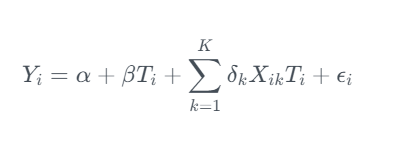
We can use Double Machine Learning to estimate CATE by interacting our control features (X) with the treatment effect in the second stage model.
User generated image
This can be really powerful as we are now able to get customer level treatment effects!
Linear Programming
What is it?
Linear programming is an optimisation method which can be used to find the optimal solution of a linear function given some constraints. It is often used to solve transportation, scheduling and resource allocation problems. A more generic term which you might see used is Operations Research.
Let’s break linear programming down with a simple example:
Decision variables: These are the unknown quantities which we want to estimate optimal values for — The marketing spend on Social Media, TV and Paid Search.
Objectives function: The linear equation we are trying to minimise or maximise — The marketing Return on Investment (ROI).
Constraints: Some restrictions on the decision variables, usually represented by linear inequalities — Total marketing spend between £100,000 and £500,000.
The intersection of all constraints forms a feasible region, which is the set of all possible solutions that satisfy the given constraints. The goal of linear programming is to find the point within the feasible region that optimizes the objective function.
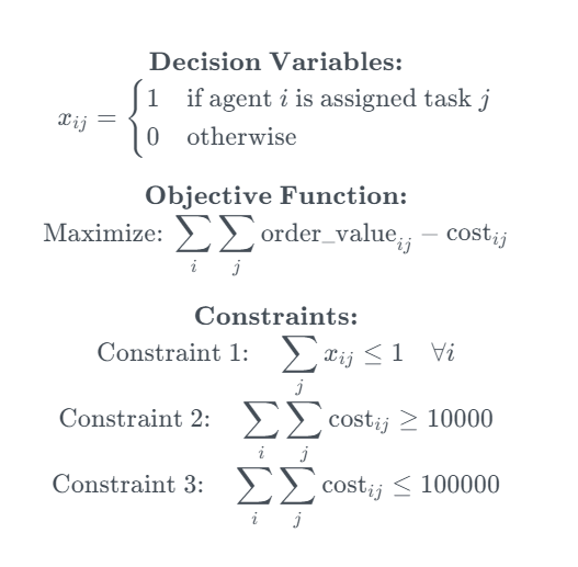
Assignment problems
Assignment problems are a specific type of linear programming problem where the goal is to assign a set of “tasks” to a set of “agents”. Lets use an example to bring it to life:
You run an experiment where you send different discounts out to 4 random groups of existing customers (the 4th of which actually you don’t send any discount). You build 2 CATE models — (1) Estimating how the offer value effects the order value and (2) Estimating how offer value effects the cost.
Agents: Your existing customer base
Tasks: Whether you send them a 10%, 20% or 50% discount
Decision variables: Binary decision variable
Objective function: The total order value minus costs
Constraint 1: Each agent is assigned to at most 1 task
Constraint 2: The cost ≥ £10,000
Constraint 3: The cost ≤ £100,000
User generated image
We basically want to find out the optimal treatment for each customer given some overall cost constraints. And linear programming can help us do this!
It is worth noting that this problem is “NP hard”, a classification of problems that are at least as hard as the hardest problems in NP (nondeterministic polynomial time).
Linear programming is a really tricky but rewarding topic. I’ve tried to introduce the idea to get us started — If you want to learn more I recommend this resource:
OR tools is an open source package developed by Google which can solve a range of linear programming problems, including assignment problems. We will demonstrate it in action later in the article.
We are going to continue with the assignment problem example and illustrate how we can solve this in Python.
Data generating process
We set up a data generating process with the following characteristics:
Difficult nuisance parameters (b)
Treatment effect heterogeneity (tau)
The X features are customer characteristics taken before the treatment:
User generated image
T is a binary flag indicating whether the customer received the offer. We create three different treatment interactions to allow us to simulate different treatment effects.
User generated image
def data_generator(tau_weight, interaction_num):
# Set number of observations n=10000
# Set number of features p=10
# Create features X = np.random.uniform(size=n * p).reshape((n, -1))
# Set treatment effect if interaction_num==1: tau = tau_weight * interaction_1 elif interaction_num==2: tau = tau_weight * interaction_2 elif interaction_num==3: tau = tau_weight * interaction_3
# Calculate outcome y = b + T * tau + np.random.normal(size=n)
return X, T, tau, y
We can use the data generator to simulate three treatments, each with a different treatment effect.
We then train three DML models using LightGBM as flexible first stage models. This should allow us to capture the difficult nuisance parameters whilst correctly calculating the treatment effect.
Pay attention to how we pass the X features in through X rather than W (unlike in the last article where we passed the X features through W). Features passed through X will be used in both the first and second stage models — In the second stage model the features are used to create interaction terms with the treatment residual.
np.random.seed(123)

# Train DML model using flexible stage 1 models
dml1 = LinearDML(model_y=LGBMRegressor(), model_t=LGBMClassifier(), discrete_treatment=True)
dml1.fit(y1, T=T1, X=X1, W=None)

# Train DML model using flexible stage 1 models
dml2 = LinearDML(model_y=LGBMRegressor(), model_t=LGBMClassifier(), discrete_treatment=True)
dml2.fit(y2, T=T2, X=X2, W=None)

# Train DML model using flexible stage 1 models
dml3 = LinearDML(model_y=LGBMRegressor(), model_t=LGBMClassifier(), discrete_treatment=True)
dml3.fit(y3, T=T3, X=X3, W=None)
When we plot the actual vs estimated CATE, we see that the model does a reasonable job.
# Create a figure and subplots fig, axes = plt.subplots(1, 3, figsize=(15, 5))
# Plot scatter plots on each subplot sns.scatterplot(x=dml1.effect(X1), y=tau1, ax=axes[0]) axes[0].set_title('Treatment 1') axes[0].set_xlabel('Estimated CATE') axes[0].set_ylabel('Actual CATE')
# Add labels to the entire figure fig.suptitle('Actual vs Estimated')
# Show plots plt.show()
User generated image
Naive optimisation
We will start by exploring this as an optimisation problem. We have a three treatments which a customer could receive. Below we create a mapping for the cost of each treatment, and set an overall cost constraint.
# Create mapping for cost of each treatment
cost_dict = {'T1': 0.1, 'T2': 0.2, 'T3': 0.3}

# Set constraints
max_cost = 3000
We can then estimate the CATE for each customer and then initially select each customers best treatment. However, selecting the best treatment doesn’t keep us within the maximum cost constraint. Therefore select the customers with the highest CATE until we reach our max cost constraint.
# Concatenate features X = np.concatenate((X1, X2, X3), axis=0)
# Estimate CATE for each treatment using DML models Treatment_1 = dml1.effect(X) Treatment_2 = dml2.effect(X) Treatment_3 = dml3.effect(X) cate = pd.DataFrame({"T1": Treatment_1, "T2": Treatment_2, "T3": Treatment_3})
# Select the best treatment for each customer best_treatment = cate.idxmax(axis=1) best_value = cate.max(axis=1)
# Map cost for each treatment best_cost = pd.Series([cost_dict[value] for value in best_treatment])
# Create dataframe with each customers best treatment and associated cost best_df = pd.concat([best_value, best_cost], axis=1) best_df.columns = ["value", "cost"] best_df = best_df.sort_values(by=['value'], ascending=False).reset_index(drop=True)
# x[i, j] is an array of 0-1 variables, which will be 1 if customer i is assigned to treatment j. x = {} for i in range(num_custs): for j in range(num_treatments): x[i, j] = solver.IntVar(0, 1, '')
# Each customer is assigned to at most 1 treatment. for i in range(num_custs): solver.Add(solver.Sum([x[i, j] for j in range(num_treatments)]) <= 1)
# Cost constraints solver.Add(sum([costs[i][j] * x[i, j] for j in range(num_treatments) for i in range(num_custs)]) <= max_cost) solver.Add(sum([costs[i][j] * x[i, j] for j in range(num_treatments) for i in range(num_custs)]) >= min_cost)
# Objective objective_terms = [] for i in range(num_custs): for j in range(num_treatments): objective_terms.append((order_value[i][j] * x[i, j] - costs[i][j] * x[i, j] )) solver.Maximize(solver.Sum(objective_terms))
# Solve status = solver.Solve()
assignments = [] values = []
if status == pywraplp.Solver.OPTIMAL or status == pywraplp.Solver.FEASIBLE: for i in range(num_custs): for j in range(num_treatments): # Test if x[i,j] is 1 (with tolerance for floating point arithmetic). if x[i, j].solution_value() > -0.5: assignments.append([i, j]) values.append([x[i, j].solution_value(), costs[i][j] * x[i, j].solution_value(), order_value[i][j]])
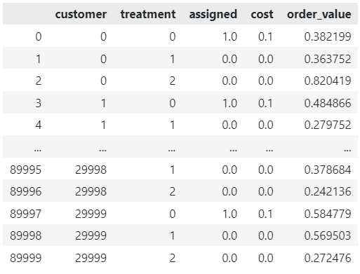
# Create a DataFrame from the collected data df = pd.DataFrame(assignments, columns=['customer', 'treatment']) df['assigned'] = [x[0] for x in values] df['cost'] = [x[1] for x in values] df['order_value'] = [x[2] for x in values]
df
User generated image
Whilst keeping to the cost constraint of £3k, we can generate £18k in order value using the optimised treatment strategy. This is 36% higher than the naive approach!
print(f'The total order value from the optimised treatment strategy is {opt_order_value} with a cost of {opt_cost_check}')
User generated image
Final thoughts
Today we covered using Double Machine Learning and Linear Programming to optimise treatment strategies. Here are some closing thoughts:
We covered Linear DML, you may want to explore alternative approaches which are more suited to dealing with complex interaction effects in the second stage model:
But also remember you don’t have to use DML, other methods like T-Learner or DR-Learner could be used.
To keep this article to a quick read I did not tune the hyper-parameters — As we increase the complexity of the problem and approach used, we need to pay closer attention to this part.
Linear programming/assignment problems are NP hard, so if you have a large customer base and/or several treatments this part of the code may take a long time to run.
It can be challenging operationalising a daily pipeline with linear programming/assignment problems — An alternative is running the optimisation periodically and learning the optimal policy based on the results in order to create a segmentation to use in a daily pipeline.
Follow me if you want to continue this journey into Causal AI — In the next article we will explore how we can estimate non-linear treatment effects in pricing and marketing optimisation problems.
Time and again, leading scientists, technologists, and philosophers have made spectacularly terrible guesses about the direction of innovation. Even Einstein was not immune, claiming, “There is not the slightest indication that nuclear energy will ever be obtainable,” just ten years before Enrico Fermi completed construction of the first fission reactor in Chicago. Shortly thereafter, the consensus switched to fears of an imminent nuclear holocaust. Similarly, today’s experts warn that an artificial general intelligence (AGI) doomsday is imminent. Others retort that large language models (LLMs) have already reached the peak of their powers. It’s difficult to argue with David Collingridge’s influential…
Paris, France, April 25th, 2024, Chainwire Prize pool of over 1M€ value including media grant from Cointelegraph Proof of Pitch is part of Proof of Talk, where All Global Leaders in Web3 Meet 10-11 June 2024, Museum of Decorative Arts (MAD), Louvre Palace, Paris In a ground-breaking shift from traditional pitch competitions, Proof of Pitch […]
We use cookies on our website to give you the most relevant experience by remembering your preferences and repeat visits. By clicking “Accept”, you consent to the use of ALL the cookies.
This website uses cookies to improve your experience while you navigate through the website. Out of these, the cookies that are categorized as necessary are stored on your browser as they are essential for the working of basic functionalities of the website. We also use third-party cookies that help us analyze and understand how you use this website. These cookies will be stored in your browser only with your consent. You also have the option to opt-out of these cookies. But opting out of some of these cookies may affect your browsing experience.
Necessary cookies are absolutely essential for the website to function properly. These cookies ensure basic functionalities and security features of the website, anonymously.
Cookie
Duration
Description
cookielawinfo-checkbox-analytics
11 months
This cookie is set by GDPR Cookie Consent plugin. The cookie is used to store the user consent for the cookies in the category "Analytics".
cookielawinfo-checkbox-functional
11 months
The cookie is set by GDPR cookie consent to record the user consent for the cookies in the category "Functional".
cookielawinfo-checkbox-necessary
11 months
This cookie is set by GDPR Cookie Consent plugin. The cookies is used to store the user consent for the cookies in the category "Necessary".
cookielawinfo-checkbox-others
11 months
This cookie is set by GDPR Cookie Consent plugin. The cookie is used to store the user consent for the cookies in the category "Other.
cookielawinfo-checkbox-performance
11 months
This cookie is set by GDPR Cookie Consent plugin. The cookie is used to store the user consent for the cookies in the category "Performance".
viewed_cookie_policy
11 months
The cookie is set by the GDPR Cookie Consent plugin and is used to store whether or not user has consented to the use of cookies. It does not store any personal data.
Functional cookies help to perform certain functionalities like sharing the content of the website on social media platforms, collect feedbacks, and other third-party features.
Performance cookies are used to understand and analyze the key performance indexes of the website which helps in delivering a better user experience for the visitors.
Analytical cookies are used to understand how visitors interact with the website. These cookies help provide information on metrics the number of visitors, bounce rate, traffic source, etc.
Advertisement cookies are used to provide visitors with relevant ads and marketing campaigns. These cookies track visitors across websites and collect information to provide customized ads.