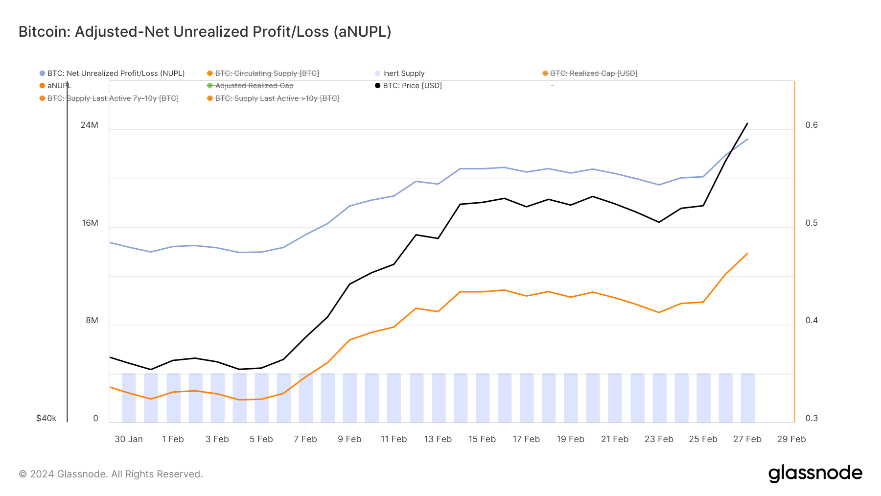
Bitcoin crossed $60,000 on Feb. 28 in a remarkable one-day candle, posting a 20% increase in just three days. However, the short stint at this level means we’ll have to wait another 24 hours before any meaningful on-chain data becomes available. However, the possibility of a correction within the next 24 hours can be analyzed, […]
Ark Invest and 21Shares have integrated Chainlink Proof of Reserve on the Ethereum mainnet to bolster transparency of the ARK 21Shares Bitcoin ETF (ARKB), according to a Feb. 28 statement. With this move, investors in ARKB can verify that the ETF’s Bitcoin holdings completely support its value. This transparency is facilitated by the public accessibility […]
MusicLM, Google’s flagship text-to-music AI, was originally published in early 2023. Even in its basic version, it represented a major breakthrough and caught the music industry by surprise. However, a few weeks ago, MusicLM received a significant update. Here’s a side-by-side comparison for two selected prompts:
Prompt: “Dance music with a melodic synth line and arpeggiation”:
This increase in quality can be attributed to a new paper by Google Research titled: “MusicRL: Aligning Music Generation to Human Preferences”. Apparently, this upgrade was considered so significant that they decided to rename the model. However, under the hood, MusicRL is identical to MusicLM in its key architecture. The only difference: Finetuning.
What is Finetuning?
When building an AI model from scratch, it starts with zero knowledge and essentially does random guessing. The model then extracts useful patterns through training on data and starts displaying increasingly intelligent behavior as training progresses. One downside to this approach is that training from scratch requires a lot of data. Finetuning is the idea that an existing model is used and adapted to a new task, or adapted to approach the same task differently. Because the model already has learned the most important patterns, much less data is required.
For example, a powerful open-source LLM like Mistral7B can be trained from scratch by anyone, in principle. However, the amount of data required to produce even remotely useful outputs is gigantic. Instead, companies use the existing Mistral7B model and feed it a small amount of proprietary data to make it solve new tasks, whether that is writing SQL queries or classifying emails.
The key takeaway is that finetuning does not change the fundamental structure of the model. It only adapts its internal logic slightly to perform better on a specific task. Now, let’s use this knowledge to understand how Google finetuned MusicLM on user data.
How Google Gathered User Data
A few months after the MusicLM paper, a public demo was released as part of Google’s AI Test Kitchen. There, users could experiment with the text-to-music model for free. However, you might know the saying: If the product is free, YOU are the product. Unsurprisingly, Google is no exception to this rule. When using MusicLM’s public demo, you were occasionally confronted with two generated outputs and asked to state which one you prefer. Through this method, Google was able to gather 300,000 user preferences within a couple of months.
Example of the user preference ratings captured in the MusicLM public playground. Image taken from the MusicRL paper.
As you can see from the screenshot, users were not explicitly informed that their preferences would be used for machine learning. While that may feel unfair, it is important to note that many of our actions in the internet are being used for ML training, whether it is our Google search history, our Instagram likes, or our private Spotify playlists. In comparison to these rather personal and sensitive cases, music preferences on the MusicLM playground seem negligible.
Example of User Data Collection on Linkedin Collaborative Articles
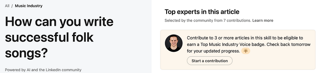
It is good to be aware that user data collection for machine learning is happening all the time and usually without explicit consent. If you are on Linkedin, you might have been invited to contribute to so-called “collaborative articles”. Essentially, users are invited to provide tips on questions in their domain of expertise. Here is an example of a collaborative article on how to write a successful folk song (something I didn’t know I needed).
Header of a collaborative article on songwriting. On the right side, I am asked to contribute to earn a “Top Voice” badge.
Users are incentivized to contribute, earning them a “Top Voice” badge on the platform. However, my impression is that noone actually reads these articles. This leads me to believe that these thousands of question-answer pairs are being used by Microsoft (owner of Linkedin) to train an expert AI system on these data. If my suspicion is accurate, I would find this example much more problematic than Google asking users for their favorite track.
But back to MusicLM!
How Google Took Advantage of this User Data
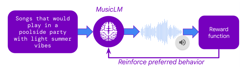
The next question is how Google was able to use this massive collection of user preferences to finetune MusicLM. The secret lies in a technique called Reinforcement Learning from Human Feedback (RLHF) which was one of the key breakthroughs of ChatGPT back in 2022. In RLHF, human preferences are used to train an AI model that learns to imitate human preference decisions, resulting in an artificial human rater. Once this so-called reward model is trained, it can take in any two tracks and predict which one would most likely be preferred by human raters.
With the reward model set up, MusicLM could be finetuned to maximize the predicted user preference of its outputs. This means that the text-to-music model generated thousands of tracks, each track receiving a rating from the reward model. Through the iterative adaptation of the model weights, MusicLM learned to generate music that the artificial human rater “likes”.
In addition to the finetuning on user preferences, MusicLM was also finetuned concerning two other criteria: 1. Prompt Adherence MuLan, Google’s proprietary text-to-audio embedding model was used to calculate the similarity between the user prompt and the generated audio. During finetuning, this adherence score was maximized. 2. Audio Quality Google trained another reward model on user data to evaluate the subjective audio quality of its generated outputs. These user data seem to have been collected in separate surveys, not in MusicLM’s public demo.
How Much Better is the New MusicLM?
The new, finetuned model seems to reliably outperform the old MusicLM, listen to the samples provided on the demo page. Of course, a selected public demo can be deceiving, as the authors are incentivized to showcase examples that make their new model look as good as possible. Hopefully, we will get to test out MusicRL in a public playground, soon.
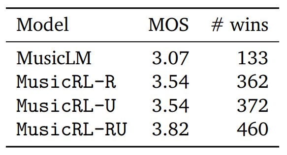
However, the paper also provides a quantitative assessment of subjective quality. For this, Google conducted a study and asked users to compare two tracks generated for the same prompt, giving each track a score from 1 to 5. Using this metric with the fancy-sounding name Mean Opinion Score (MOS), we can compare not only the number of direct comparison wins for each model, but also calculate the average rater score (MOS).
Quantitative benchmarks. Image taken from MusicRL paper.
Here, MusicLM represents the original MusicLM model. MusicRL-R was only finetuned for audio quality and prompt adherence. MusicRL-U was finetuned solely on human feedback (the reward model). Finally, MusicRL-RU was finetuned on all three objectives. Unsurprisingly, MusicRL-RU beats all other models in direct comparison as well as on the average ratings.
The paper also reports that MusicRL-RU, the fully finetuned model, beat MusicLM in 87% of direct comparisons. The importance of RLHF can be shown by analyzing the direct comparisons between MusicRL-R and MusicRL-RU. Here, the latter had a 66% win rate, reliably outperforming its competitor.
What are the Implications of This?
Although the difference in output quality is noticeable, qualitatively as well as quantitatively, the new MusicLM is still quite far from human-level outputs in most cases. Even on the public demo page, many generated outputs sound odd, rhythmically, fail to capture key elements of the prompt or suffer from unnatural-sounding instruments.
In my opinion, this paper is still significant, as it is the first attempt at using RLHF for music generation. RLHF has been used extensively in text generation for more than one year. But why has this taken so long? I suspect that collecting user feedback and finetuning the model is quite costly. Google likely released the public MusicLM demo with the primary intention of collecting user feedback. This was a smart move and gave them an edge over Meta, which has equally capable models, but no open platform to collect user data on.
All in all, Google has pushed itself ahead of the competition by leveraging proven finetuning methods borrowed from ChatGPT. While even with RLHF, the new MusicLM has still not reached human-level quality, Google can now maintain and update its reward model, improving future generations of text-to-music models with the same finetuning procedure.
It will be interesting to see if and when other competitors like Meta or Stability AI will be catching up. For us as users, all of this is just great news! We get free public demos and more capable models.
For musicians, the pace of the current developments may feel a little threatening — and for good reason. I expect to see human-level text-to-music generation in the next 1–3 years. By that, I mean text-to-music AI that is at least as capable at producing music as ChatGPT was at writing texts when it was released. Musicians must learn about AI and how it can already support them in their everyday work. As the music industry is being disrupted once again, curiosity and flexibility will be the primary key to success.
Interested in Music AI?
If you liked this article, you might want to check out some of my other work:
Histograms are widely used and easily grasped, but when it comes to estimating continuous densities, people often resort to treating it as a mysterious black box. However, understanding this concept is just as straightforward and becomes crucial, especially when dealing with bounded data like age, height, or price, where available libraries may not handle it automatically.
1. Kernel Density Estimation
Histogram
A histogram involves partitioning the data range into bins or sub-intervals and counting the number of samples that fall within each bin. It thus approximates the continuous density function with a piecewise constant function.
Large bin size: It helps capturing the low-frequency outline of the density function, by gathering neighboring samples to avoid empty bins. However, it looses the continuity property because there could be a significant gap between the count of adjacent bins.
Small bin size: It helps capturing details at higher frequencies. However, if the number of samples is too small, we’ll end up with lots of empty bins at places where the true density isn’t.
Histogram of 100 samples drawn from a Gaussian Distribution, with increasing number of bins (5/10/50)— Image by the author
Kernel Density Estimation (KDE)
An intuitive idea is to assume that the density function from which the samples are drawn is smooth, and leverage it to fill-in the gaps of our high frequency histogram.
This is precisely what the Kernel Density Estimation (KDE) does. It estimates the global density as the average of local density kernels K centered around each sample. A Kernel is a non-negative function integrating to 1, e.g uniform, triangular, normal… Just like adjusting the bin size in a histogram, we introduce a bandwidth parameter h that modulates the deviation of the kernel around each sample point. It thus controls the smoothness of the resulting density estimate.
Bandwith Selection
Finding the right balance between under- and over-smoothing isn’t straightforward. A popular and easy-to-compute heuristic is the Silverman’s rule of thumb, which is optimal when the underlying density being estimated is Gaussian.
Silverman’s Rule of thumb, with n the number of samples and sigma the standard deviation of the samples
Keep in mind that it may not always yield optimal results across all data distributions. I won’t discuss them in this article, but there are other alternatives and improvements available.
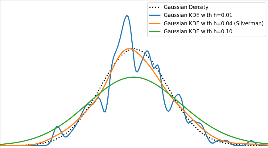
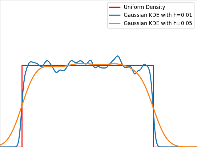
The image below depicts a Gaussian distribution being estimated by a gaussian KDE at different bandwidth values. As we can see, Silverman’s rule of thumb is well-suited, but higher bandwidths cause over-smoothing, while lower ones introduce high-frequency oscillations around the true density.
Gaussian Kernel Density Estimation from 100 samples drawn from a true gaussian distribution, for different bandwith parameters (0.01, 0.04, 0.10) — Image by the author
Examples
The video below illustrates the convergence of a Kernel Density Estimation with a Gaussian kernel across 4 standard density distributions as the number of provided samples increases.
Although it’s not optimal, I’ve chosen to keep a small constant bandwidth h over the video to better illustrate the process of kernel averaging, and to prevent excessive smoothing when the sample size is very small.
Convergence of Gaussian Kernel Density Estimation across 4 Standard Density Distributions (Uniform, Triangular, Gaussian, Gaussian Mixture) with Increasing Sample Size. — Video by the author
Implementation of Gaussian Kernel Density Estimation
Great python libraries like scipy and scikit-learn provide public implementations for Kernel Density Estimation:
scipy.stats.gaussian_kde
sklearn.neighbors.KernelDensity
However, it’s valuable to note that a basic equivalent can be built in just three lines using numpy. We need the samples x_data drawn from the distribution to estimate and the points x_prediction at which we want to evaluate the density estimate. Then, using array broadcasting we can evaluate a local gaussian kernel around each input sample and average them into the final density estimate.
N.B. This version is fast because it’s vectorized. However it involves creating a large 2D temporary array of shape (len(x_data), len(x_prediction)) to store all the kernel evaluations. To have a lower memory footprint, we could re-write it using numba or cython (to avoid the computational burden of Python for loops) to aggregate kernel evaluations on-the-fly in a running sum for each output prediction.
Real-life data is often bounded by a given domain. For example, attributes such as age, weight, or duration are always non-negative values. In such scenarios, a standard smooth KDE may fail to accurately capture the true shape of the distribution, especially if there’s a density discontinuity at the boundary.
In 1D, with the exception of some exotic cases, bounded distributions typically have either one-sided (e.g. positive values) or two-sided (e.g. uniform interval) bounded domains.
As illustrated in the graph below, kernels are bad at estimating the edges of the uniform distribution and leak outside the bounded domain.
Gaussian KDE on 100 samples drawn from a uniform distribution — Image by the author
No Clean Public Solution in Python
Unfortunately, popular public Python libraries like scipy and scikit-learn do not currently address this issue. There are existing GitHub issues and pull requests discussing this topic, but regrettably, they have remained unresolved for quite some time.
In R, kde.boundary allows Kernel density estimate for bounded data.
There are various ways to take into account the bounded nature of the distribution. Let’s describe the most popular ones: Reflection, Weighting and Transformation.
Warning: For the sake of readability, we will focus on the unit bounded domain, i.e. [0,1]. Please remember to standardize the data and scale the density appropriately in the general case [a,b].
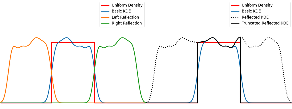
Solution: Reflection
The trick is to augment the set of samples by reflecting them across the left and right boundaries. This is equivalent to reflecting the tails of the local kernels to keep them in the bounded domain. It works best when the density derivative is zero at the boundary.
The reflection technique also implies processing three times more sample points.
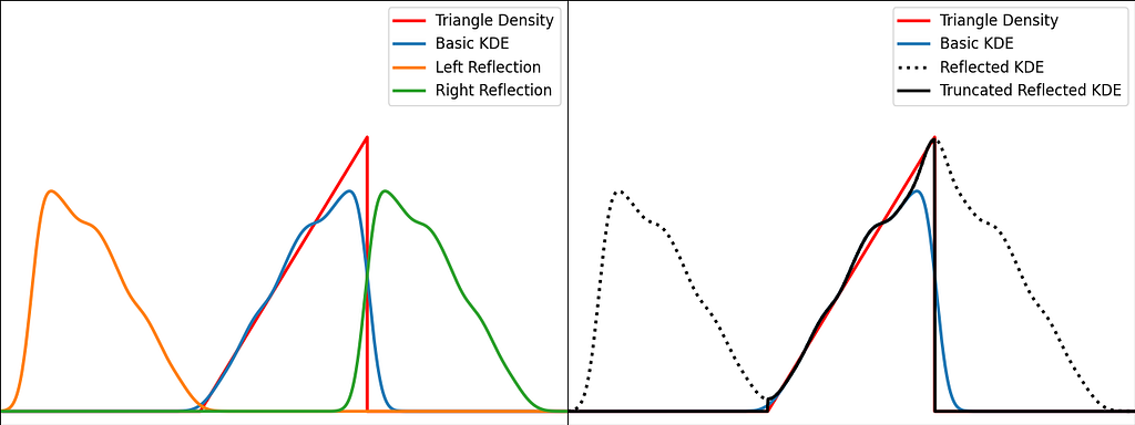
The graphs below illustrate the reflection trick for three standard distributions: uniform, right triangle and inverse square root. It does a pretty good job at reducing the bias at the boundaries, even for the singularity of the inverse square root distribution.
KDE on an uniform distribution, using reflections to handle boundaries— Image by the authorKDE on a triangle distribution, using reflections to handle boundaries — Image by the authorKDE on an inverse square root distribution, using reflections to handle boundaries — Image by the author
N.B. The signature of basic_kde has been slightly updated to allow to optionally provide your own bandwidth parameter instead of using the Silverman’s rule of thumb.
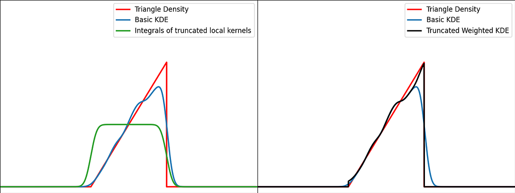
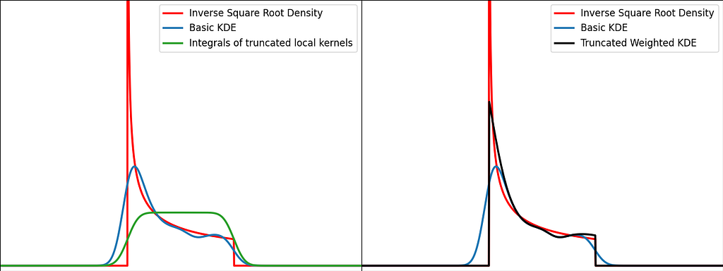
Solution: Weighting
The reflection trick presented above takes the leaking tails of the local kernel and add them back to the bounded domain, so that the information isn’t lost. However, we could also compute how much of our local kernel has been lost outside the bounded domain and leverage it to correct the bias.
For a very large number of samples, the KDE converges to the convolution between the kernel and the true density, truncated by the bounded domain.
If x is at a boundary, then only half of the kernel area will actually be used. Intuitively, we’d like to normalize the convolution kernel to make it integrate to 1 over the bounded domain. The integral will be close to 1 at the center of the bounded interval and will fall off to 0.5 near the borders. This accounts for the lack of neighboring kernels at the boundaries.
Similarly to the reflection technique, the graphs below illustrate the weighting trick for three standard distributions: uniform, right triangle and inverse square root. It performs very similarly to the reflection method.
From a computational perspective, it doesn’t require to process 3 times more samples, but it needs to evaluate the normal Cumulative Density Function at the prediction points.
KDE on an uniform distribution, applying weight on the sides to handle boundaries — Image by the authorKDE on a triangular distribution, applying weight on the sides to handle boundaries — Image by the authorKDE on an inverse square root distribution, applying weight on the sides to handle boundaries — Image by the author
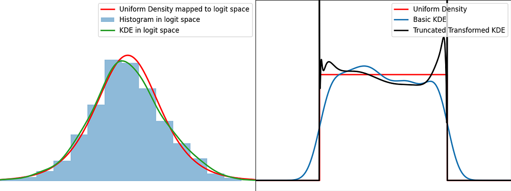
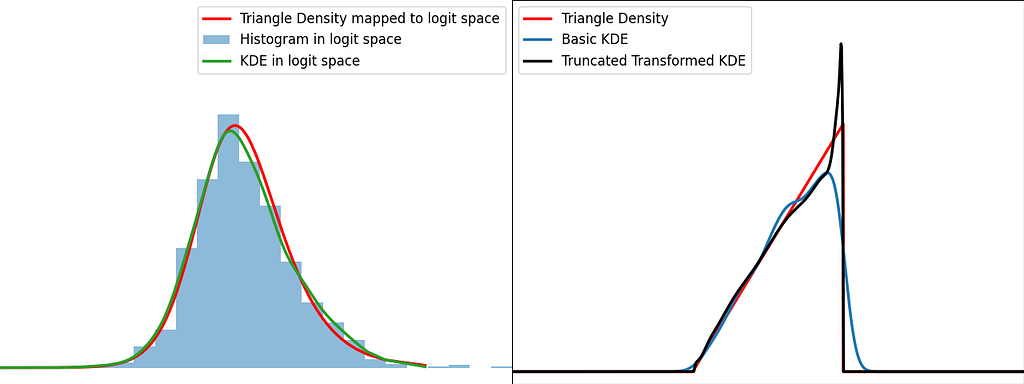
Transformation
The transformation trick maps the bounded data to an unbounded space, where the KDE can be safely applied. This results in using a different kernel function for each input sample.
The logit function leverages the logarithm to map the unit interval [0,1] to the entire real axis.
Logit function — Image by the author
When applying a transform f onto a random variable X, the resulting density can be obtained by dividing by the absolute value of the derivative of f.
We can now apply it for the special case of the logit transform to retrieve the density distribution from the one estimated in the logit space.
Similarly to the reflection and weighting techniques, the graphs below illustrate the weighting trick for three standard distributions: uniform, right triangle and inverse square root. It performs quite poorly by creating large oscillations at the boundaries. However, it handles extremely well the singularity of the inverse square root.
KDE on an uniform distribution, computed after mapping the samples to the logit space — Image by the authorKDE on a triangular distribution, computed after mapping the samples to the logit space — Image by the authorKDE on an inverse square root distribution, computed after mapping the samples to the logit space— Image by the authorPhoto by Martin Martz on Unsplash
Conclusion
Histograms and KDE
In Kernel Density Estimation, each sample is assigned its own local kernel density centered around it, and then we average all these densities to obtain the global density. The bandwidth parameter defines how far the influence of each kernel extends. Intuitively, we should decrease the bandwidth as the number of samples increases, to prevent excessive smoothing.
Histograms can be seen as a simplified version of KDE. Indeed, the bins implicitly define a finite set of possible rectangular kernels, and each sample is assigned to the closest one. Finally, the average of all these densities result in a piecewise-constant estimate of the global density.
Which method is the best ?
Reflection, weighting and transform are efficient basic methods to handle bounded data during KDE. However, bear in mind that there isn’t a one-size-fits-all solution; it heavily depends on the shape of your data.
The transform method handles pretty well the singularities, as we’ve seen with the inverse square root distribution. As for reflection and weighting, they are generally more suitable for a broader range of scenarios.
Reflection introduces complexity during training, whereas weighting adds complexity during inference.
From [0,1] to [a,b], [a, +∞[ and ]-∞,b]
Code presented above has been written for data bounded in the unit interval. Don’t forget to scale the density, when applying the affine transformation to normalize your data.
It can also easily be adjusted for a one-sided bounded domain, by reflecting only on one side, integrating the kernel to infinity on one side or using the logarithm instead of logit.
I hope you enjoyed reading this article and that it gave you more insights on how Kernel Density Estimation works and how to handle bounded domains!
Decoding the Math behind Q-Learning, Action-Value Functions, and Bellman Equations, and building them from scratch in Python.
Image Generated by DALLE
In the previous article, we dipped our toes into the world of reinforcement learning (RL), covering the basics like how agents learn from their surroundings, focusing on a simple setup called GridWorld. We went over the essentials — actions, states, rewards, and how to get around in this environment. If you’re new to this or need a quick recap, it might be a good idea to check out that piece again to get a firm grip on the basics before diving in deeper.
Today, we’re ready to take it up a bit. We will explore more complex aspects of RL, moving from simple setups to dynamic, ever-changing environments and more sophisticated ways for our agents to navigate through them. We’ll dive into the concept of the Markov Decision Process, which is very important for understanding how RL works at a deeper level. Plus, we’ll take a closer look at Q-learning, a key algorithm in RL that shows how agents can learn to make smart decisions in places like GridWorld, even when things are constantly changing.
When we first started exploring reinforcement learning (RL), we looked at simple, unchanging worlds. But as we move to dynamic environments, things get a lot more interesting. Unlike static setups where everything stays the same, dynamic environments are all about change. Obstacles move, goals shift, and rewards vary, making these settings much closer to the real world’s unpredictability.
What Makes Dynamic Environments Special? Dynamic environments are key for teaching agents to adapt because they mimic the constant changes we face daily. Here, agents need to do more than just find the quickest route to a goal; they have to adjust their strategies as obstacles move, goals relocate, and rewards increase or decrease. This continuous learning and adapting are what could lead to true artificial intelligence.
Moving back to the environment we created in the last article, GridWorld, a 5×5 board with obstacles inside it. In this article, we’ll add some complexity to it making the obstacles shuffle randomly.
The Impact of Dynamic Environments on RL Agents Dynamic environments train RL agents to be more robust and intelligent. Agents learn to adjust their strategies on the fly, a skill critical for navigating the real world where change is the only constant.
Facing a constantly evolving set of challenges, agents must make more nuanced decisions, balancing the pursuit of immediate rewards against the potential for future gains. Moreover, agents trained in dynamic environments are better equipped to generalize their learning to new, unseen situations, a key indicator of intelligent behavior.
2: Markov Decision Process
2.1: Understanding MDP
Before we dive into Q-Learning, let’s introduce the Markov Decision Process, or MDP for short. Think of MDP as the ABC of reinforcement learning. It offers a neat framework for understanding how an agent decides and learns from its surroundings. Picture MDP like a board game. Each square is a possible situation (state) the agent could find itself in, the moves it can make (actions), and the points it racks up after each move (rewards). The main aim is to collect as many points as possible.
Differing from the classic RL framework we introduced in the previous article, which focused on the concepts of states, actions, and rewards in a broad sense, MDP adds structure to these concepts by introducing transition probabilities and the optimization of policies. While the classic framework sets the stage for understanding reinforcement learning, MDP dives deeper, offering a mathematical foundation that accounts for the probabilities of moving from one state to another and optimizing the decision-making process over time. This detailed approach helps bridge the gap between theoretical learning and practical application, especially in environments where outcomes are partly uncertain and partly under the agent’s control.
Transition Probabilities Ideally, we’d know exactly what happens next after an action. But life, much like MDP, is full of uncertainties. Transition probabilities are the rules that predict what comes next. If our game character jumps, will they land safely or fall? If the thermostat is cranked up, will the room get to the desired temperature?
Now imagine a maze game, where the agent aims to find the exit. Here, states are its spots in the maze, actions are which way it moves, and rewards come from exiting the maze with fewer moves.
MDP frames this scenario in a way that helps an RL agent figure out the best moves in different states to max out rewards. By playing this “game” repeatedly, the agent learns which actions work best in each state to score the highest, despite the uncertainties.
2.2: The Math Behind MDP
To get what the Markov Decision Process is about in reinforcement learning, it’s key to dive into its math. MDP gives us a solid setup for figuring out how to make decisions when things aren’t totally predictable and there’s some room for choice. Let’s break down the main math bits and pieces that paint the full picture of MDP.
Core Components of MDP MDP is characterized by a tuple (S, A, P, R, γ), where:
S is a set of states,
A is a set of actions,
P is the state transition probability matrix,
R is the reward function, and
γ is the discount factor.
While we covered the math behind states, actions, and the discount factor in the previous article, now we’ll introduce the math behind the state transition probability, and the reward function.
State Transition Probabilities The state transition probability P(s′ ∣ s, a) defines the probability of transitioning from state s to state s′ after taking action a. This is a core element of the MDP that captures the dynamics of the environment. Mathematically, it’s expressed as:
State Transition Probabilities Formula — Image by Author
Here:
s: The current state of the agent before taking the action.
a: The action taken by the agent in state s.
s′: The subsequent state the agent finds itself in after action a is taken.
P(s′ ∣ s, a): The probability that action a in state s will lead to state s′.
Pr denotes the probability, St represents the state at time t.
St+1 is the state at time t+1 after the action At is taken at time t.
This formula captures the essence of the stochastic nature of the environment. It acknowledges that the same action taken in the same state might not always lead to the same outcome due to the inherent uncertainties in the environment.
Consider a simple grid world where an agent can move up, down, left, or right. If the agent tries to move right, there might be a 90% chance it successfully moves right (s′=right), a 5% chance it slips and moves up instead (s′=up), and a 5% chance it slips and moves down (s′=down). There’s no probability of moving left since it’s the opposite direction of the intended action. Hence, for the action a=right from state s, the state transition probabilities might look like this:
P(right ∣ s, right) = 0.9
P(up ∣ s, right) = 0.05
P(down ∣ s, right) = 0.05
P(left ∣ s, right) = 0
Understanding and calculating these probabilities are fundamental for the agent to make informed decisions. By anticipating the likelihood of each possible outcome, the agent can evaluate the potential rewards and risks associated with different actions, guiding it towards decisions that maximize expected returns over time.
In practice, while exact state transition probabilities might not always be known or directly computable, various RL algorithms strive to estimate or learn these dynamics to achieve optimal decision-making. This learning process lies at the core of an agent’s ability to navigate and interact with complex environments effectively.
Reward Function The reward function R(s, a, s′) specifies the immediate reward received after transitioning from state s to state s′ as a result of taking action a. It can be defined in various ways, but a common form is:
Reward Function — Image by Author
Here:
Rt+1: This is the reward received at the next time step after taking the action, which could vary depending on the stochastic elements of the environment.
St=s: This indicates the current state at time t.
At=a: This is the action taken by the agent in state s at time t.
St+1=s′: This denotes the state at the next time step t+1 after the action a has been taken.
E[Rt+1 ∣ St=s, At=a, St+1=s′]: This represents the expected reward after taking action a in state s and ending up in state s′. The expectation E is taken over all possible outcomes that could result from the action, considering the probabilistic nature of the environment.
In essence, this function calculates the average or expected reward that the agent anticipates receiving for making a particular move. It takes into account the uncertain nature of the environment, as the same action in the same state may not always lead to the same next state or reward because of the probabilistic state transitions.
For example, if an agent is in a state representing its position in a grid, and it takes an action to move to another position, the reward function will calculate the expected reward of that move. If moving to that new position means reaching a goal, the reward might be high. If it means hitting an obstacle, the reward might be low or even negative. The reward function encapsulates the goals and rules of the environment, incentivizing the agent to take actions that will maximize its cumulative reward over time.
Policies A policy π is a strategy that the agent follows, where π(a ∣ s) defines the probability of taking action a in state s. A policy can be deterministic, where the action is explicitly defined for each state, or stochastic, where actions are chosen according to a probability distribution:
Policy Function — Image by Author
π(a∣s): The probability that the agent takes action a given it is in state s.
Pr(At=a∣St=s): The conditional probability that action a is taken at time t given the current state at time t is s.
Let’s consider a simple example of an autonomous taxi navigating in a city. Here the states are the different intersections within a city grid, and the actions are the possible maneuvers at each intersection, like ‘turn left’, ‘go straight’, ‘turn right’, or ‘pick up a passenger’.
The policy π might dictate that at a certain intersection (state), the taxi has the following probabilities for each action:
π(’turn left’∣intersection) = 0.1
π(’go straight’∣intersection) = 0.7
π(’turn right’∣intersection) = 0.1
π(’pick up passenger’∣intersection) = 0.1
In this example, the policy is stochastic because there are probabilities associated with each action rather than a single certain outcome. The taxi is most likely to go straight but has a small chance of taking other actions, which may be due to traffic conditions, passenger requests, or other variables.
The policy function guides the agent in selecting actions that it believes will maximize the expected return or reward over time, based on its current knowledge or strategy. Over time, as the agent learns, the policy may be updated to reflect new strategies that yield better results, making the agent’s behavior more sophisticated and better at achieving its goals.
Value Functions Once I have my set of states, actions, and policies defined, we could ask ourselves the following question
What rewards can I expect in the long run if I start here and follow my game plan?
The answer is in the value function Vπ(s), which gives the expected return when starting in state s and following policy π thereafter:
Value Functions — Image by Author
Where:
Vπ(s): The value of state s under policy π.
Gt: The total discounted return from time t onwards.
Eπ[Gt∣St=s]: The expected return starting from state s following policy π.
γ: The discount factor between 0 and 1, which determines the present value of future rewards — a way of expressing that immediate rewards are more certain than distant rewards.
Rt+k+1: The reward received at time t+k+1, which is k steps in the future.
∑k=0∞: The sum of the discounted rewards from time t onward.
Imagine a game where you have a grid with different squares, and each square is a state that has different points (rewards). You have a policy π that tells you the probability of moving to other squares from your current square. Your goal is to collect as many points as possible.
For a particular square (state s), the value function Vπ(s) would be the expected total points you could collect from that square, discounted by how far in the future you receive them, following your policy π for moving around the grid. If your policy is to always move to the square with the highest immediate points, then Vπ(s) would reflect the sum of points you expect to collect, starting from s and moving to other squares according to π, with the understanding that points available further in the future are worth slightly less than points available right now (due to the discount factor γ).
In this way, the value function helps to quantify the long-term desirability of states given a particular policy, and it plays a key role in the agent’s learning process to improve its policy.
Action-Value Function This function goes a step further, estimating the expected return of taking a specific action in a specific state and then following the policy. It’s like saying:
If I make this move now and stick to my strategy, what rewards am I likely to see?
While the value function V(s) is concerned with the value of states under a policy without specifying an initial action. In contrast, the action-value function Q(s, a) extends this concept to evaluate the value of taking a particular action in a state, before continuing with the policy.
The action-value function Qπ(s, a) represents the expected return of taking action a in state s and following policy π thereafter:
Action-Value Function — Image by Author
Qπ(s, a): The value of taking action a in state s under policy π.
Gt: The total discounted return from time t onward.
Eπ[Gt ∣ St=s, At=a]: The expected return after taking action a in state s the following policy π.
γ: The discount factor, which determines the present value of future rewards.
Rt+k+1: The reward received k time steps in the future, after action a is taken at time t.
∑k=0∞: The sum of the discounted rewards from time t onward.
The action-value function tells us what the expected return is if we start in state s, take action a, and then follow policy π after that. It takes into account not only the immediate reward received for taking action a but also all the future rewards that follow from that point on, discounted back to the present time.
Let’s say we have a robot vacuum cleaner with a simple task: clean a room and return to its charging dock. The states in this scenario could represent the vacuum’s location within the room, and the actions might include ‘move forward’, ‘turn left’, ‘turn right’, or ‘return to dock’.
The action-value function Qπ(s, a) helps the vacuum determine the value of each action in each part of the room. For instance:
Qπ(middle of the room, ’move forward’) would represent the expected total reward the vacuum would get if it moves forward from the middle of the room and continues cleaning following its policy π.
Qπ(near the dock, ’return to dock’) would represent the expected total reward for heading back to the charging dock to recharge.
The action-value function will guide the vacuum to make decisions that maximize its total expected rewards, such as cleaning as much as possible before needing to recharge.
In reinforcement learning, the action-value function is central to many algorithms, as it helps to evaluate the potential of different actions and informs the agent on how to update its policy to improve its performance over time.
2.3: The Math Behind Bellman Equations
In the world of Markov Decision Processes, the Bellman equations are fundamental. They act like a map, helping us navigate through the complex territory of decision-making to find the best strategies or policies. The beauty of these equations is how they simplify big challenges — like figuring out the best move in a game — into more manageable pieces.
They lay down the groundwork for what an optimal policy looks like — the strategy that maximizes rewards over time. They’re especially crucial in algorithms like Q-learning, where the agent learns the best actions through trial and error, adapting even when faced with unexpected situations.
Bellman Equation for Vπ(s) This equation computes the expected return (total future rewards) of being in state s under a policy π. It sums up all the rewards an agent can expect to receive, starting from state s, and taking into account the likelihood of each subsequent state-action pair under the policy π. Essentially, it answers, “If I follow this policy, how good is it to be in this state?”
Bellman Equation for Vπ(s) — Image by Author
π(a∣s) is the probability of taking action a in state s under policy π.
P(s′ ∣ s, a) is the probability of transitioning to state s′ from state s after taking action a.
R(s, a, s′) is the reward received after transitioning from s to s′ due to action a.
γ is the discount factor, which values future rewards less than immediate rewards (0 ≤ γ < 1).
Vπ(s′) is the value of the subsequent state s′.
This equation calculates the expected value of a state s by considering all possible actions a, the likelihood of transitioning to a new state s′, the immediate reward R(s, a, s′), plus the discounted value of the subsequent state s′. It encapsulates the essence of planning under uncertainty, emphasizing the trade-offs between immediate rewards and future gains.
Bellman Equation for Qπ(s,a) This equation goes a step further by evaluating the expected return of taking a specific action a in state s, and then following policy π afterward. It provides a detailed look at the outcomes of specific actions, giving insights like, “If I take this action in this state and then stick to my policy, what rewards can I expect?”
Bellman Equation for Qπ(s,a) — Image by Author
P(s′ ∣ s, a) and R(s, a, s′) are as defined above.
γ is the discount factor.
π(a′ ∣ s′) is the probability of taking action a′ in the next state s′ under policy π.
Qπ(s′, a′) is the value of taking action a′ in the subsequent state s′.
This equation extends the concept of the state-value function by evaluating the expected utility of taking a specific action a in a specific state s. It accounts for the immediate reward and the discounted future rewards obtained by following policy π from the next state s′ onwards.
Both equations highlight the relationship between the value of a state (or a state-action pair) and the values of subsequent states, providing a way to evaluate and improve policies.
While value functions V(s) and action-value functions Q(s, a) represent the core objectives of learning in reinforcement learning — estimating the value of states and actions — the Bellman equations provide the recursive framework necessary for computing these values and enabling the agent to improve its decision-making over time.
3: Deep Dive into Q-Learning
Now that we’ve established all the foundational knowledge necessary for Q-Learning, let’s dive into action!
3.1: Fundamentals of Q-Learning
Image Generated by DALLE
Q-learning works through trial and error. In particular, the agent checks out its surroundings, sometimes randomly picking paths to discover new ways to go. After it makes a move, the agent sees what happens and what kind of reward it gets. A good move, like getting closer to the goal, earns a positive reward. A not-so-good move, like smacking into a wall, means a negative reward. Based on what it learns, the agent updates its guide, bumping up the scores for good moves and lowering them for the bad ones. As the agent keeps exploring and updating its guide, it gets sharper at picking the best moves.
Let’s use the prior robot vacuum example. A Q-learning powered robot vacuum may firstly move around randomly. But as it keeps at it, it learns from the outcomes of its moves.
For instance, if moving forward means it cleans up a lot of dust (earning a high reward), the robot notes that going forward in that spot is a great move. If turning right causes it to bump into a chair (getting a negative reward), it learns that turning right there isn’t the best option.
The “cheat sheet” the robot builds is what Q-learning is all about. It’s a bunch of values (known as Q-values) that help guide the robot’s decisions. The higher the Q-value for a particular action in a specific situation, the better that action is. Over many cleaning rounds, the robot keeps refining its Q-values with every move it makes, constantly improving its cheat sheet until it nails down the best way to clean the room and zip back to its charger.
3.2: The Math Behind Q-Learning
Q-learning is a model-free reinforcement learning algorithm that seeks to find the best action to take given the current state. It’s about learning a function that will give us the best action to maximize the total future reward.
The Q-learning Update Rule: A Mathematical Formula The mathematical heart of Q-learning lies in its update rule, which iteratively improves the Q-values that estimate the returns of taking certain actions from particular states. Here is the Q-learning update rule expressed in mathematical terms:
Q-Learning Update Formula — Image by Author
Let’s break down the components of this formula:
Q(s, a): The current Q-value for a given state s and action a.
α: The learning rate, a factor that determines how much new information overrides old information. It is a number between 0 and 1.
R(s, a): The immediate reward received after taking action a in state s.
γ: The discount factor, also a number between 0 and 1, which discounts the value of future rewards compared to immediate rewards.
maxa′Q(s′, a′): The maximum predicted reward for the next state s′, achieved by any action a′. This is the agent’s best guess at how valuable the next state will be.
Q(s, a): The old Q-value before the update.
The essence of this rule is to adjust the Q-value for the state-action pair towards the sum of the immediate reward and the discounted maximum reward for the next state. The agent does this after every action it takes, slowly honing its Q-values towards the true values that reflect the best possible decisions.
The Q-values are initialized arbitrarily, and then the agent interacts with its environment, making observations, and updating its Q-values according to the rule above. Over time, with enough exploration of the state-action space, the Q-values converge to the optimal values, which reflect the maximum expected return one can achieve from each state-action pair.
This convergence means that the Q-values eventually provide the agent with a strategy for choosing actions that maximize the total expected reward for any given state. The Q-values essentially become a guide for the agent to follow, informing it of the value or quality of taking each action when in each state, hence the name “Q-learning”.
Difference with Bellman Equation Comparing the Bellman Equation for Qπ(s, a) with the Q-learning update rule, we see that Q-learning essentially applies the Bellman equation in a practical, iterative manner. The key differences are:
Learning from Experience: Q-learning uses the observed immediate reward R(s, a) and the estimated value of the next state maxa′Q(s′, a′) directly from experience, rather than relying on the complete model of the environment (i.e., the transition probabilities P(s′ ∣ s, a)).
Temporal Difference Learning: Q-learning’s update rule reflects a temporal difference learning approach, where the Q-values are updated based on the difference (error) between the estimated future rewards and the current Q-value.
4: Q-Learning From Scratch
To better understand every step of Q-Learning beyond its math, let’s build it from scratch. Take a look first at the whole code we will be using to create a reinforcement learning setup using a grid world environment and a Q-learning agent. The agent learns to navigate through the grid, avoiding obstacles and aiming for a goal.
Don’t worry if the code doesn’t seem clear, as we will break it down and go through it in detail later.
The code below is also accessible through this GitHub repo:
import numpy as np import matplotlib.pyplot as plt import matplotlib.animation as animation import pickle import os
# GridWorld Environment class GridWorld: """GridWorld environment with obstacles and a goal. The agent starts at the top-left corner and has to reach the bottom-right corner. The agent receives a reward of -1 at each step, a reward of -0.01 at each step in an obstacle, and a reward of 1 at the goal.
Args: size (int): The size of the grid. num_obstacles (int): The number of obstacles in the grid.
Attributes: size (int): The size of the grid. num_obstacles (int): The number of obstacles in the grid. obstacles (list): The list of obstacles in the grid. state_space (numpy.ndarray): The state space of the grid. state (tuple): The current state of the agent. goal (tuple): The goal state of the agent.
Methods: generate_obstacles: Generate the obstacles in the grid. step: Take a step in the environment. reset: Reset the environment. """ def __init__(self, size=5, num_obstacles=5): self.size = size self.num_obstacles = num_obstacles self.obstacles = [] self.generate_obstacles() self.state_space = np.zeros((self.size, self.size)) self.state = (0, 0) self.goal = (self.size-1, self.size-1)
def generate_obstacles(self): """ Generate the obstacles in the grid. The obstacles are generated randomly in the grid, except in the top-left and bottom-right corners.
Args: None
Returns: None """ for _ in range(self.num_obstacles): while True: obstacle = (np.random.randint(self.size), np.random.randint(self.size)) if obstacle not in self.obstacles and obstacle != (0, 0) and obstacle != (self.size-1, self.size-1): self.obstacles.append(obstacle) break
def step(self, action): """ Take a step in the environment. The agent takes a step in the environment based on the action it chooses.
Args: action (int): The action the agent takes. 0: up 1: right 2: down 3: left
Returns: state (tuple): The new state of the agent. reward (float): The reward the agent receives. done (bool): Whether the episode is done or not. """ x, y = self.state if action == 0: # up x = max(0, x-1) elif action == 1: # right y = min(self.size-1, y+1) elif action == 2: # down x = min(self.size-1, x+1) elif action == 3: # left y = max(0, y-1) self.state = (x, y) if self.state in self.obstacles: return self.state, -1, True if self.state == self.goal: return self.state, 1, True return self.state, -0.01, False
def reset(self): """ Reset the environment. The agent is placed back at the top-left corner of the grid.
Args: None
Returns: state (tuple): The new state of the agent. """ self.state = (0, 0) return self.state
# Q-Learning class QLearning: """ Q-Learning agent for the GridWorld environment.
Args: env (GridWorld): The GridWorld environment. alpha (float): The learning rate. gamma (float): The discount factor. epsilon (float): The exploration rate. episodes (int): The number of episodes to train the agent.
Attributes: env (GridWorld): The GridWorld environment. alpha (float): The learning rate. gamma (float): The discount factor. epsilon (float): The exploration rate. episodes (int): The number of episodes to train the agent. q_table (numpy.ndarray): The Q-table for the agent.
Methods: choose_action: Choose an action for the agent to take. update_q_table: Update the Q-table based on the agent's experience. train: Train the agent in the environment. save_q_table: Save the Q-table to a file. load_q_table: Load the Q-table from a file. """ def __init__(self, env, alpha=0.5, gamma=0.95, epsilon=0.1, episodes=10): self.env = env self.alpha = alpha self.gamma = gamma self.epsilon = epsilon self.episodes = episodes self.q_table = np.zeros((self.env.size, self.env.size, 4))
def choose_action(self, state): """ Choose an action for the agent to take. The agent chooses an action based on the epsilon-greedy policy.
Args: state (tuple): The current state of the agent.
Returns: action (int): The action the agent takes. 0: up 1: right 2: down 3: left """ if np.random.uniform(0, 1) < self.epsilon: return np.random.choice([0, 1, 2, 3]) # exploration else: return np.argmax(self.q_table[state]) # exploitation
def update_q_table(self, state, action, reward, new_state): """ Update the Q-table based on the agent's experience. The Q-table is updated based on the Q-learning update rule.
Args: state (tuple): The current state of the agent. action (int): The action the agent takes. reward (float): The reward the agent receives. new_state (tuple): The new state of the agent.
def train(self): """ Train the agent in the environment. The agent is trained in the environment for a number of episodes. The agent's experience is stored and returned.
Args: None
Returns: rewards (list): The rewards the agent receives at each step. states (list): The states the agent visits at each step. starts (list): The start of each new episode. steps_per_episode (list): The number of steps the agent takes in each episode. """ rewards = [] states = [] # Store states at each step starts = [] # Store the start of each new episode steps_per_episode = [] # Store the number of steps per episode steps = 0 # Initialize the step counter outside the episode loop episode = 0 while episode < self.episodes: state = self.env.reset() total_reward = 0 done = False while not done: action = self.choose_action(state) new_state, reward, done = self.env.step(action) self.update_q_table(state, action, reward, new_state) state = new_state total_reward += reward states.append(state) # Store state steps += 1 # Increment the step counter if done and state == self.env.goal: # Check if the agent has reached the goal starts.append(len(states)) # Store the start of the new episode rewards.append(total_reward) steps_per_episode.append(steps) # Store the number of steps for this episode steps = 0 # Reset the step counter episode += 1 return rewards, states, starts, steps_per_episode
def save_q_table(self, filename): """ Save the Q-table to a file.
Args: filename (str): The name of the file to save the Q-table to.
Returns: None """ filename = os.path.join(os.path.dirname(__file__), filename) with open(filename, 'wb') as f: pickle.dump(self.q_table, f)
def load_q_table(self, filename): """ Load the Q-table from a file.
Args: filename (str): The name of the file to load the Q-table from.
Returns: None """ filename = os.path.join(os.path.dirname(__file__), filename) with open(filename, 'rb') as f: self.q_table = pickle.load(f)
# Initialize environment and agent for i in range(10): env = GridWorld(size=5, num_obstacles=5) agent = QLearning(env)
# Load the Q-table if it exists if os.path.exists(os.path.join(os.path.dirname(__file__), 'q_table.pkl')): agent.load_q_table('q_table.pkl')
# Train the agent and get rewards rewards, states, starts, steps_per_episode = agent.train() # Get starts and steps_per_episode as well
# Save the Q-table agent.save_q_table('q_table.pkl')
# Visualize the agent moving in the grid fig, ax = plt.subplots()
def update(i): """ Update the grid with the agent's movement.
Args: i (int): The current step.
Returns: None """ ax.clear() # Calculate the cumulative reward up to the current step cumulative_reward = sum(rewards[:i+1]) # Find the current episode current_episode = next((j for j, start in enumerate(starts) if start > i), len(starts)) - 1 # Calculate the number of steps since the start of the current episode if current_episode < 0: steps = i + 1 else: steps = i - starts[current_episode] + 1 ax.set_title(f"Iteration: {current_episode+1}, Total Reward: {cumulative_reward:.2f}, Steps: {steps}") grid = np.zeros((env.size, env.size)) for obstacle in env.obstacles: grid[obstacle] = -1 grid[env.goal] = 1 grid[states[i]] = 0.5 # Use states[i] instead of env.state ax.imshow(grid, cmap='cool')
ani = animation.FuncAnimation(fig, update, frames=range(len(states)), repeat=False)
# After the animation print(f"Environment number {i+1}") for i, steps in enumerate(steps_per_episode, 1): print(f"Iteration {i}: {steps} steps") print(f"Total reward: {sum(rewards):.2f}") print()
plt.show()
That was a lot of code! Let’s break down this code into smaller, more understandable steps. Here’s what each part does:
4.1: The GridWorld Environment
This class represents a grid environment where an agent can move around, avoid obstacles, and reach a goal.
When you create a new GridWorld, you specify the size of the grid and the number of obstacles. The grid is square, so size=5 means a 5×5 grid. The agent starts at the top-left corner (0, 0) and aims to reach the bottom-right corner (size-1, size-1). The obstacles are held in self.obstacles, which is an empty list of obstacles that will be filled with the locations of the obstacles. The generate_obstacles() method is then called to randomly place obstacles in the grid.
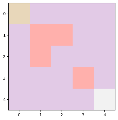
Therefore, we could expect an environment like the following:
Environment — Image by Author
In the environment above the top-left block is the starting state, the bottom-right block is the goal, and the pink blocks in the middle are the obstacles. Note that the obstacles will vary everytime you create an environment, as they are generated randomly.
Generating Obstacles (generate_obstacles method)
def generate_obstacles(self):
    for _ in range(self.num_obstacles):
        while True:
            obstacle = (np.random.randint(self.size), np.random.randint(self.size))
            if obstacle not in self.obstacles and obstacle != (0, 0) and obstacle != (self.size-1, self.size-1):
                self.obstacles.append(obstacle)
                  break
This method places num_obstacles randomly within the grid. It ensures that obstacles don’t overlap with the starting point or the goal.
It does this by looping until the specified number of obstacles ( self.num_obstacles)have been placed. In every loop, it randomly selects a position in the grid, then if the position is not already an obstacle, and not the start or goal, it’s added to the list of obstacles.
Taking a Step (step method)
def step(self, action):
    x, y = self.state
    if action == 0:  # up
        x = max(0, x-1)
    elif action == 1:  # right
        y = min(self.size-1, y+1)
    elif action == 2:  # down
        x = min(self.size-1, x+1)
    elif action == 3:  # left
        y = max(0, y-1)
    self.state = (x, y)
    if self.state in self.obstacles:
        return self.state, -1, True
    if self.state == self.goal:
        return self.state, 1, True
    return self.state, -0.01, False
The step method moves the agent according to the action (0 for up, 1 for right, 2 for down, 3 for left) and updates its state. It also checks the new position to see if it’s an obstacle or a goal.
It does that by taking the current state (x, y), which is the current location of the agent. Then, it changes x or y based on the action (0 for up, 1 for right, 2 for down, 3 for left), ensuring the agent doesn’t move outside the grid boundaries. It updates self.state to this new position. Then it checks if the new state is an obstacle or the goal and returns the corresponding reward and whether the episode is finished (done).
When you create a QLearning agent, you provide it with the environment to learn from self.env, which is the GridWorld environment in our case; a learning rate alpha, which controls how new information affects the existing Q-values; a discount factor gamma, which determines the importance of future rewards; an exploration rate epsilon, which controls the trade-off between exploration and exploitation.
Then, we also initialize the number of episodes for training. The Q-table, which stores the agent’s knowledge, and it’s a 3D numpy array of zeros with dimensions (env.size, env.size, 4), representing the Q-values for each state-action pair. 4 is the number of possible actions the agent can take in every state.
The agent picks an action based on the epsilon-greedy policy. Most of the time, it chooses the best-known action (exploitation), but sometimes it randomly explores other actions.
Here, epsilon is the probability a random action is chosen. Otherwise, the action with the highest Q-value for the current state is chosen (argmax over the Q-values).
In our example, we set epsilon it to 0.1, which means that the agent will take a random action 10% of the time. Therefore, when np.random.uniform(0,1) generating a number lower than 0.1, a random action will be taken. This is done to prevent the agent from being stuck on a suboptimal strategy, and instead going out and exploring before being set on one.
After the agent takes an action, it updates its Q-table with the new knowledge. It adjusts the value of the action based on the immediate reward and the discounted future rewards from the new state.
It updates the Q-table using the Q-learning update rule. It modifies the value for the state-action pair in the Q-table (self.q_table[state][action]) based on the received reward and the estimated future rewards (using np.max(self.q_table[new_state]) for the future state).
Training the Agent (train method)
def train(self):
    rewards = []
    states = []  # Store states at each step
    starts = []  # Store the start of each new episode
    steps_per_episode = []  # Store the number of steps per episode
    steps = 0  # Initialize the step counter outside the episode loop
    episode = 0
    while episode < self.episodes:
        state = self.env.reset()
        total_reward = 0
        done = False
        while not done:
            action = self.choose_action(state)
            new_state, reward, done = self.env.step(action)
            self.update_q_table(state, action, reward, new_state)
            state = new_state
            total_reward += reward
            states.append(state)  # Store state
            steps += 1  # Increment the step counter
            if done and state == self.env.goal:  # Check if the agent has reached the goal
                starts.append(len(states))  # Store the start of the new episode
                rewards.append(total_reward)
                steps_per_episode.append(steps)  # Store the number of steps for this episode
                steps = 0  # Reset the step counter
                episode += 1
    return rewards, states, starts, steps_per_episode
This function is pretty straightforward, it runs the agent through many episodes using a while loop. In every episode, it first resets the environment by placing the agent in the starting state (0,0). Then, it chooses actions, updates the Q-table, and keeps track of the total rewards and steps it takes.
Saving and Loading the Q-Table (save_q_table and load_q_table methods)
def save_q_table(self, filename):
    filename = os.path.join(os.path.dirname(__file__), filename)
    with open(filename, 'wb') as f:
        pickle.dump(self.q_table, f)

def load_q_table(self, filename):
    filename = os.path.join(os.path.dirname(__file__), filename)
    with open(filename, 'rb') as f:
        self.q_table = pickle.load(f)
These methods are used to save the learned Q-table to a file and load it back. They use the pickle module to serialize (pickle.dump) and deserialize (pickle.load) the Q-table, allowing the agent to resume learning without starting from scratch.
Running the Simulation
Finally, the script initializes the environment and the agent, optionally loads an existing Q-table, and then starts the training process. After training, it saves the updated Q-table. There’s also a visualization section that shows the agent moving through the grid, which helps you see what the agent has learned.
Initialization
Firstly, the environment and agent are initialized:
Here, a GridWorld of size 5×5 with 5 obstacles is created. Then, a QLearning agent is initialized using this environment.
Loading and Saving the Q-table If there’s a Q-table file already saved (‘q_table.pkl’), it’s loaded, which allows the agent to continue learning from where it left off:
if os.path.exists(os.path.join(os.path.dirname(__file__), 'q_table.pkl')):
    agent.load_q_table('q_table.pkl')
After the agent is trained for the specified number of episodes, the updated Q-table is saved:
agent.save_q_table('q_table.pkl')
This ensures that the agent’s learning is not lost and can be used in future training sessions or actual navigation tasks.
Training the Agent The agent is trained by calling the train method, which runs through the specified number of episodes, allowing the agent to explore the environment, update its Q-table, and track its progress:
During training, the agent chooses actions, updates the Q-table, observes rewards, and keeps track of states visited. All of this information is used to adjust the agent’s policy (i.e., the Q-table) to improve its decision-making over time.
Visualization
After training, the code uses matplotlib to create an animation showing the agent’s journey through the grid. It visualizes how the agent moves, where the obstacles are, and the path to the goal:
fig, ax = plt.subplots()
def update(i):
    # Update the grid visualization based on the agent's current state
    ax.clear()
    # Calculate the cumulative reward up to the current step
    cumulative_reward = sum(rewards[:i+1])
    # Find the current episode
    current_episode = next((j for j, start in enumerate(starts) if start > i), len(starts)) - 1
    # Calculate the number of steps since the start of the current episode
    if current_episode < 0:
        steps = i + 1
    else:
        steps = i - starts[current_episode] + 1
    ax.set_title(f"Iteration: {current_episode+1}, Total Reward: {cumulative_reward:.2f}, Steps: {steps}")
    grid = np.zeros((env.size, env.size))
    for obstacle in env.obstacles:
        grid[obstacle] = -1
    grid[env.goal] = 1
    grid[states[i]] = 0.5  # Use states[i] instead of env.state
    ax.imshow(grid, cmap='cool')
ani = animation.FuncAnimation(fig, update, frames=range(len(states)), repeat=False)
plt.show()
This visualization is not only a nice way to see what the agent has learned, but it also provides insight into the agent’s behavior and decision-making process.
By running this simulation multiple times (as indicated by the loop for i in range(10):), the agent can have multiple learning sessions, which can potentially lead to improved performance as the Q-table gets refined with each iteration.
Now try this code out, and check how many steps it takes for the agent to reach the goal by iteration. Furthermore, try to increase the size of the environment, and see how this affects the performance.
5: Next Steps and Future Directions
As we take a step back to evaluate our journey with Q-learning and the GridWorld setup, it’s important to appreciate our progress but also to note where we hit snags. Sure, we’ve got our agents moving around a basic environment, but there are a bunch of hurdles we still need to jump over to kick their skills up a notch.
5.1: Current Problems and Limitations
Limited Complexity Right now, GridWorld is pretty basic and doesn’t quite match up to the messy reality of the world around us, which is full of unpredictable twists and turns.
Scalability Issues When we try to make the environment bigger or more complex, our Q-table (our cheat sheet of sorts) gets too bulky, making Q-learning slow and a tough nut to crack.
One-Size-Fits-All Rewards We’re using a simple reward system — dodging obstacles losing points, and reaching the goal and gaining points. But we’re missing out on the nuances, like varying rewards for different actions that could steer the agent more subtly.
Discrete Actions and States Our current Q-learning vibe works with clear-cut states and actions. But life’s not like that; it’s full of shades of grey, requiring more flexible approaches.
Lack of Generalization Our agent learns specific moves for specific situations without getting the knack for winging it in scenarios it hasn’t seen before or applying what it knows to different but similar tasks.
5.2: Next Steps
Policy Gradient Methods Policy gradient methods represent a class of algorithms in reinforcement learning that optimize the policy directly. They are particularly well-suited for problems with:
High-dimensional or continuous action spaces.
The need for fine-grained control over the actions.
Complex environments where the agent must learn more abstract concepts.
The next article will cover everything necessary to understand and implement policy gradient methods.
We’ll start with the conceptual underpinnings of policy gradient methods, explaining how they differ from value-based approaches and their advantages.
We’ll dive into algorithms like REINFORCE and Actor-Critic methods, exploring how they work and when to use them. We’ll discuss the exploration strategies used in policy gradient methods, which are crucial for effective learning in complex environments.
A key challenge with policy gradients is high variance in the updates. We will look into techniques like baselines and advantage functions to tackle this issue.
A More Complex Environment To truly harness the power of policy gradient methods, we will introduce a more complex environment. This environment will have a continuous state and action space, presenting a more realistic and challenging learning scenario. Multiple paths to success, require the agent to develop nuanced strategies. The possibility of more dynamic elements, such as moving obstacles or changing goals.
Stay tuned as we prepare to embark on this exciting journey into the world of policy gradient methods, where we’ll empower our agents to tackle challenges of increasing complexity and closer to real-world applications.
6: Conclusion
As we conclude this article, it’s clear that the journey through the fundamentals of reinforcement learning has set a robust stage for our next foray into the field. We’ve seen our agent start from scratch, learning to navigate the straightforward corridors of the GridWorld, and now it stands on the brink of stepping into a world that’s richer and more reflective of the complexities it must master.
It was a lot, but you made it to the end. Congrats! I hope you enjoyed this article. If so consider leaving a clap and following me, as I will regularly post similar articles. Let me know what you think about the article, what you would like to see more. Consider leaving a clap or two and follow me to stay updated.
We use cookies on our website to give you the most relevant experience by remembering your preferences and repeat visits. By clicking “Accept”, you consent to the use of ALL the cookies.
This website uses cookies to improve your experience while you navigate through the website. Out of these, the cookies that are categorized as necessary are stored on your browser as they are essential for the working of basic functionalities of the website. We also use third-party cookies that help us analyze and understand how you use this website. These cookies will be stored in your browser only with your consent. You also have the option to opt-out of these cookies. But opting out of some of these cookies may affect your browsing experience.
Necessary cookies are absolutely essential for the website to function properly. These cookies ensure basic functionalities and security features of the website, anonymously.
Cookie
Duration
Description
cookielawinfo-checkbox-analytics
11 months
This cookie is set by GDPR Cookie Consent plugin. The cookie is used to store the user consent for the cookies in the category "Analytics".
cookielawinfo-checkbox-functional
11 months
The cookie is set by GDPR cookie consent to record the user consent for the cookies in the category "Functional".
cookielawinfo-checkbox-necessary
11 months
This cookie is set by GDPR Cookie Consent plugin. The cookies is used to store the user consent for the cookies in the category "Necessary".
cookielawinfo-checkbox-others
11 months
This cookie is set by GDPR Cookie Consent plugin. The cookie is used to store the user consent for the cookies in the category "Other.
cookielawinfo-checkbox-performance
11 months
This cookie is set by GDPR Cookie Consent plugin. The cookie is used to store the user consent for the cookies in the category "Performance".
viewed_cookie_policy
11 months
The cookie is set by the GDPR Cookie Consent plugin and is used to store whether or not user has consented to the use of cookies. It does not store any personal data.
Functional cookies help to perform certain functionalities like sharing the content of the website on social media platforms, collect feedbacks, and other third-party features.
Performance cookies are used to understand and analyze the key performance indexes of the website which helps in delivering a better user experience for the visitors.
Analytical cookies are used to understand how visitors interact with the website. These cookies help provide information on metrics the number of visitors, bounce rate, traffic source, etc.
Advertisement cookies are used to provide visitors with relevant ads and marketing campaigns. These cookies track visitors across websites and collect information to provide customized ads.