Layer 2 network Optimism unveiled its fourth airdrop, targeting web3 artists with a generous distribution of over 10 million OP tokens, valued at approximately $40.8 million.
VanEck’s spot Bitcoin ETF jumped 14 times its daily average volume a day before the firm plans to implement a fee cut, reducing entry cost from 0.25% to 0.2%.
A year has passed since the Toloka Visual Question Answering (VQA) Challenge at the WSDM Cup 2023, and as we predicted back then, the winning machine-learning solution didn’t match up to the human baseline. However, this past year has been packed with breakthroughs in Generative AI. It feels like every other article flips between pointing out what OpenAI’s GPT models can’t do and praising what they do better than us.
Since autumn 2023, GPT-4 Turbo has gained “vision” capabilities, meaning it accepts images as input and it can now directly participate in VQA challenges. We were curious to test its ability against the human baseline in our Toloka challenge, wondering if that gap has finally closed.
Visual Question Answering
Visual Question Answering (VQA) is a multi-disciplinary artificial intelligence research problem, concentrated on making AI interpret images and answer related questions in natural language. This area has various applications: aiding visually impaired individuals, enriching educational content, supporting image search capabilities, and providing video search functionalities.
The development of VQA “comes with great responsibility”, such as ensuring the reliability and safety of the technology application. With AI systems having vision capabilities, the potential for misinformation increases, considering claims that images paired with false information can make statements appear more credible.
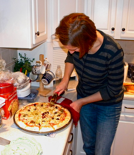
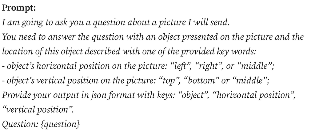
In the Toloka VQA Challenge, the task was to identify a single object and put it in a bounding box, based on a question that describes the object’s functions rather than its visual characteristics. For example, instead of asking to find something round and red, a typical question might be “What object in the picture is good in a salad and on a pizza?” This reflects the ability of humans to perceive objects in terms of their utility. It’s like being asked to find “a thing to swat a fly with” when you see a table with a newspaper, a coffee mug, and a pair of glasses — you’d know what to pick without a visual description of the object.
Question: What do we use to cut the pizza into slices?
Considering this vast gap between human and AI solutions, we were very curious to see how GPT-4V would perform in the Toloka VQA Challenge. Since the challenge was based on the MS COCO dataset, used countless times in Computer Vision (for example, in the Visual Spatial Reasoning dataset), and, therefore, likely “known” to GPT-4 from its training data, there was a possibility that GPT-4V might come closer to the human baseline.
GPT-4V and Toloka VQA Challenge
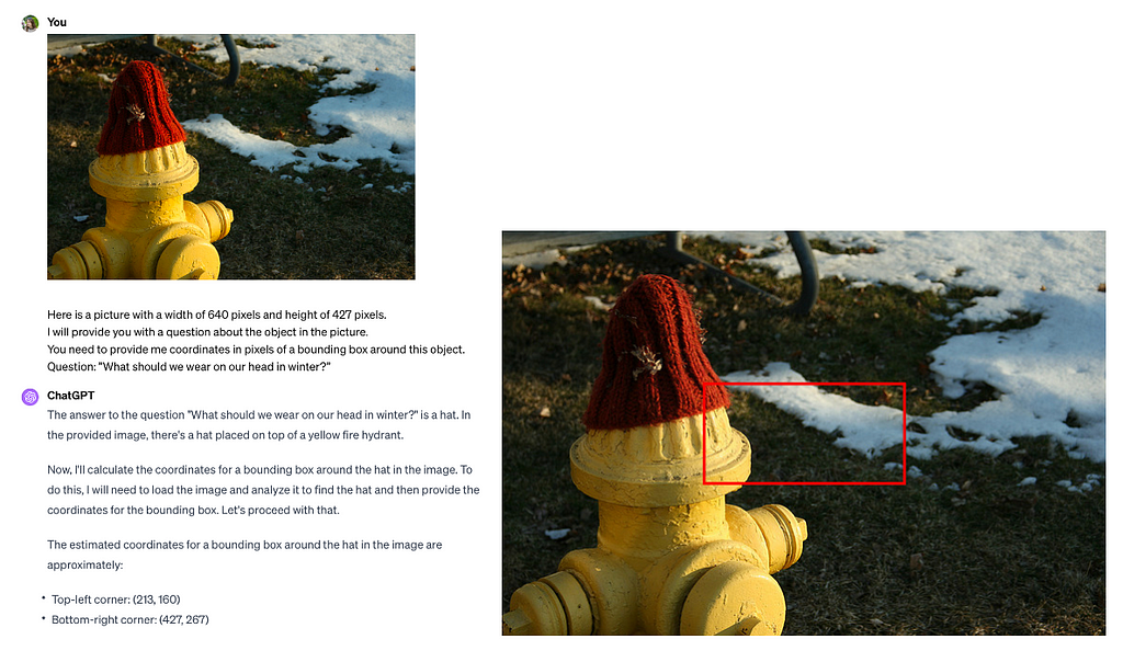
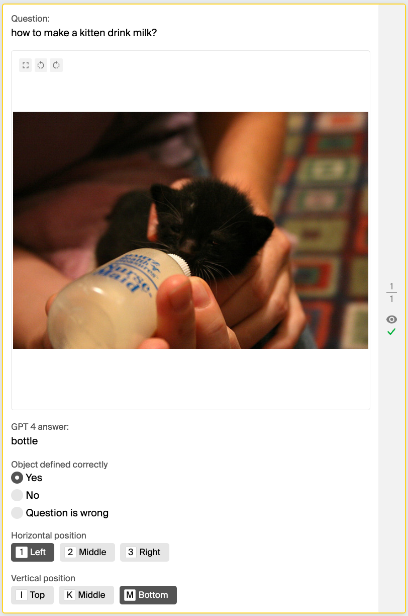
Initially, we wanted to find out if GPT-4V could handle the Toloka VQA Challenge as is.
However, even though GPT-4V mostly defined the object correctly, it had serious trouble providing meaningful coordinates for bounding boxes. This wasn’t entirely unexpected since OpenAI’s guide acknowledges GPT-4V’s limitations in tasks that require identifying precise spatial localization of an object on an image.
Image by author
This led us to explore how well GPT-4 handles the identification of basic high-level locations in an image. Can it figure out where things are — not exactly, but if they’re on the left, in the middle, or on the right? Or at the top, in the middle, or at the bottom? Since these aren’t precise locations, it might be doable for GPT-4V, especially since it’s been trained on millions of images paired with captions pointing out the object’s directional locations. Educational materials often describe pictures in detail (just think of textbooks on brain structure that mention parts like “dendrites” at the “top left” or “axons” at the “bottom right” of an image).
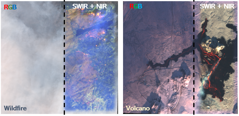
The understanding of LLM’s and MLM’s spatial reasoning limitations, even simple reasoning like we discussed above, is crucial in practical applications. The integration of GPT-4V into the “Be My Eyes” application, which assists visually impaired users by interpreting images, perfectly illustrates this importance. Despite the abilities of GPT-4V, the application advises caution, highlighting the technology’s current inability to fully substitute for human judgment in critical safety and health contexts. However, exact topics where the technology is unable to perform well are not pointed out explicitly.
GPT-4V and spatial reasoning
For our exploration into GPT-4V’s reasoning on basic locations of objects on images, we randomly chose 500 image-question pairs from a larger set of 4,500 pairs, the competition’s private test dataset. We tried to minimize the chances of our test data leaking to the training data of GPT-4V since this subset of the competition data was released the latest in the competition timeline.
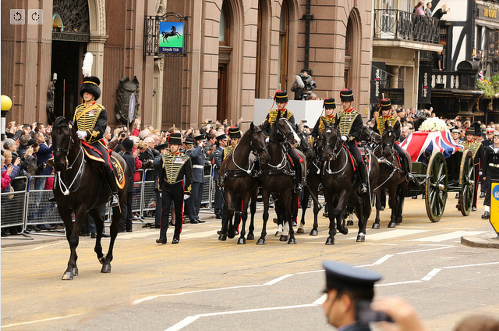
Out of these 500 pairs, 25 were rejected by GPT-4V, flagged as ‘invalid image’. We suspect this rejection was due to built-in safety measures, likely triggered by the presence of objects that could be classified as Personally Identifiable (PI) information, such as peoples’ faces. The remaining 475 pairs were used as the basis for our experiments.
Take an example pair with a lampshade above, sampled from the experiment data. One person might say it’s towards the top-left of the image because the lampshade leans a bit left, while another might call it middle-top, seeing it centered in the picture. Both views have a point. It’s tough to make strict rules for identifying locations because objects can have all kinds of shapes and parts, like a lamp’s long cord, which might change how we see where it’s placed.
Keeping this complexity in mind, we planned to try out at least two different methods for labeling the ground truth of where things are in an image.
It works in the following way: if the difference in pixels between the center of the image and the center of the object (marked by its bounding box) is less than or equal to a certain percentage of the image’s width (for horizontal position) or height (for vertical position), then we label the object as being in the middle. If the difference is more, it gets labeled as either left or right (or top or bottom). We settled on using 2% as the threshold percentage. This decision was based on observing how this difference appeared for objects of various sizes relative to the overall size of the image.
object_horizontal_center = bb_left + (bb_right - bb_left) / 2
image_horizontal_center = image_width / 2
difference = object_horizontal_center - image_horizontal_center
if difference > (image_width * 0.02):
    return 'right'
else if difference < (-1 * image_width * 0.02):
    return 'left'
else:
    return 'middle'For our first approach, we decided on simple automated heuristics to figure out where objects are placed in a picture, both horizontally and vertically. This idea came from an assumption that GPT-4V might use algorithms found in publicly available code for tasks of a similar nature.
For the second approach, we used labeling with crowdsourcing. Here are the details on how the crowdsourcing project was set up:
Images were shown to the crowd without bounding boxes to encourage less biased (on a ground truth answer) labeling of an object’s location, as one would in responding to a query regarding the object’s placement in a visual context.
GPT-4V’s answers were displayed as both a hint and a way to validate its object detection accuracy.
Participants had the option to report if a question couldn’t be clearly answered with the given image, removing any potential ambiguous/grey-zone cases from the dataset.
To ensure the quality of the crowdsourced responses, I reviewed all instances where GPT-4’s answers didn’t match the crowd’s. I couldn’t see either GPT-4V’s or the crowd’s responses during this review process, which allowed me to adjust the labels without preferential bias.
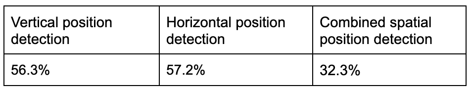
We opted for accuracy as our evaluation metric because the classes in our dataset were evenly distributed. After evaluating GPT-4V’s performance against the ground truth — established through crowdsourcing and heuristic methods — on 475 images, we excluded 45 pairs that the crowd found difficult to answer. The remaining data revealed that GPT-4V’s accuracy in identifying both horizontal and vertical positions was remarkably low, at around 30%, when compared to both the crowdsourced and heuristic labels.
Accuracy of GPT-4V’s answers compared to automated heuristicsAccuracy of GPT-4V’s answers compared to crowd labeling
Even when we accepted GPT-4V’s answer as correct if it matched either the crowdsourced or heuristic approach, its accuracy still didn’t reach 50%, resulting in 40.2%.
To further validate these findings, we manually reviewed 100 image-question pairs that GPT-4V had incorrectly labeled.
By directly asking GPT-4V to specify the objects’ locations and comparing its responses, we confirmed the initial results.
GPT-4V consistently confused left and right, top and bottom, so if GPT-4V is your navigator, be prepared to take the scenic route — unintentionally.
However, GPT-4V’s object recognition capabilities are impressive, achieving an accuracy rate of 88.84%. This suggests that by integrating GPT-4V with specialized object detection tools, we could potentially match (or even exceed) the human baseline. This is the next objective of our research.
Prompt engineering & directional dyslexia
To ensure we’re not pointing out the limitations of GPT-4V without any prompt optimization efforts, so as not to become what we hate, we explored various prompt engineering techniques mentioned in the research literature as ones enhancing spatial reasoning in LLMs.
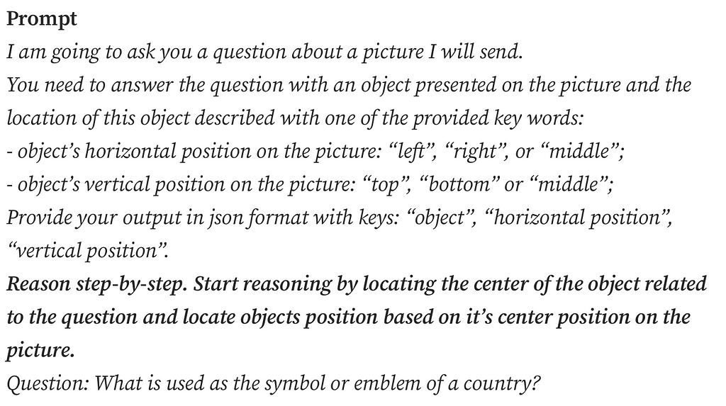
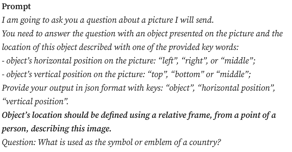
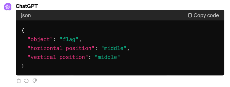
Question: What is used as the symbol or emblem of a country?
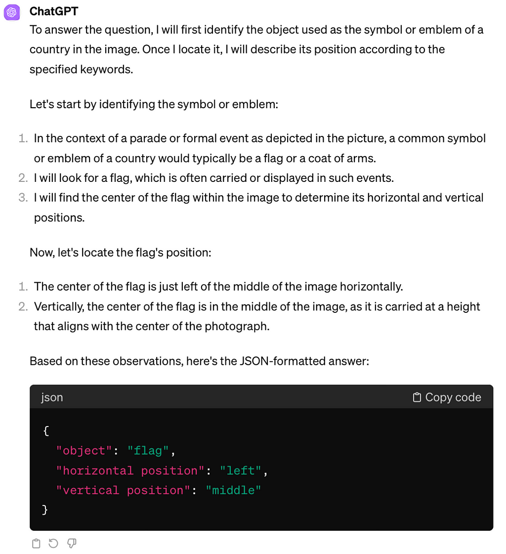
We applied three discovered prompt engineering techniques on the experimental dataset example above that GPT-4V stubbornly and consistently misinterpreted. The flag which is asked about is located in the middle-right of the picture.
The “Shikra: Unleashing Multimodal LLM’s Referential Dialogue Magic” paper introduces a method combining Chain of Thought (CoT) with position annotations, specifically center annotations, called Grounding CoT (GCoT). In the GCoT setting, the authors prompt the model to provide CoT along with center points for each mentioned object. Since the authors specifically trained their model to provide coordinates of objects on an image, we had to adapt the prompt engineering technique to a less strict setting, asking the model to provide reasoning about the object’s location based on the center of the object.
Image by author. Grounding CoT approach (correct answer is middle-right)
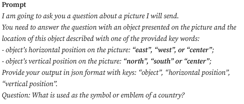
The study “Mapping Language Models to Grounded Conceptual Spaces” by Patel & Pavlick (2022) illustrates that GPT-3 can grasp spatial and cardinal directions even within a text-based grid by ‘orienting’ the models with specific word forms learned during training. They substitute traditional directional terms using north/south and west/east instead of top/bottom and left/right, to guide the model’s spatial reasoning.
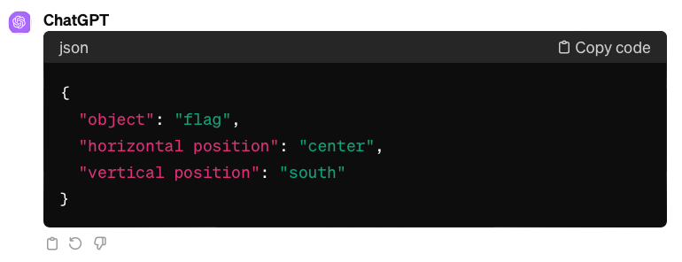
Image by author. Cardinal directions approach (correct answer is east-south)
Lastly, the “Visual Spatial Reasoning” article states the significance of different perspectives in spatial descriptions: the intrinsic frame centered on an object (e.g. behind the chair = side with a backrest), the relative frame from the viewer’s perspective, and the absolute frame using fixed coordinates (e.g. “north” of the chair). English typically favors the relative frame, so we explicitly mentioned it in the prompt, hoping to refine GPT-4V’s spatial reasoning.
Image by author. Relative frame approach (correct answer is middle-right)
As we can see from the examples, GPT-4V’s challenges with basic spatial reasoning persist.
Conclusions and future work
GPT-4V struggles with simple spatial reasoning, like identifying object horizontal and vertical positions on a high level in images. Yet its strong object recognition skills based just on implicit functional descriptions are promising. Our next step is to combine GPT-4V with models specifically trained for object detection in images. Let’s see if this combination can beat the human baseline in the Toloka VQA challenge!
How to solve binary classification problems using Bayesian methods in Python.
Bayesian Thinking — OpenAI DALL-E Generated Image by Author
Introduction
In this article, I will build a simple Bayesian logistic regression model using Pyro, a Python probabilistic programming package. This article will cover EDA, feature engineering, model build and evaluation. The focus is to provide a simple framework for Bayesian logistic regression. Therefore, the depth of the first two sections will be limited. The code used in this article can be found here:
I am using the heart failure prediction dataset from Kaggle, linked below. This dataset is provided under the Open Data Commons Open Database License (ODbL) v1.0. Full reference to this dataset can be found at the end of this article.
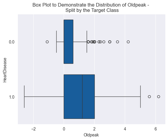
This dataset contains 918 examples and 11 features for predicting heart disease. The target variable is ‘HeartDisease’. There are five numeric and six categorical features in this dataset. To explore the distributions of the numeric features, I generated boxplots using seaborn, such as the one below.
Box plot of the feature OldPeak — Image by Author
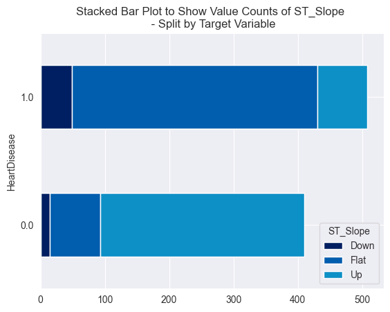
Something to highlight is the presence of outliers in the boxplot above. Outliers were present in many of the numeric features. This is important to note as it will influence the feature scaling method used in the next section. For categorical variables, I produced bar plots containing the volume of each category split by the target class.
Box plot of the feature ST_Slope — Image by Author
These graphs indicate that both of these variables could be predictive, given the difference in distribution by the target variable, ‘HeartDisease’.
Feature Engineering
I used standardisation scaling for continuous numerical features and one-hot encoding for categorical features for this model. My decision to use this scaling method was due to the presence of outliers in the features. Normalisation scaling is more sensitive to outliers, therefore employing the technique would require using methods to handle the outliers, or to remove them completely. For simplicity, I opted to use standardisation scaling, which is less sensitive to outliers.
Test and Training Data
I split the data into training and test sets using an 80/20 split. The function below generates the training and test data. Note that data is returned as PyTorch tensors.
Building the Logistic Regression Model
The function below defines the logistic regression model.
The code above generates two priors. We generate a sample of weights and a bias variable which are drawn from Normal distributions. The weights of the logistic regression model are drawn from a standard multivariate normal distribution, with a mean of 0 and a standard deviation of 1. The .independent() method is applied to the normal distribution which samples the model weights. This method tells Pyro that every sample drawn along the 1st dimension is independent. In other words, the coefficient applied to each feature in the model is independent of each other. Within the pyro.plate() context manager, the raw model logits are generated. This is calculated by the standard linear regression equation, defined below. The .squeeze() method is applied to remove dimensions that are of size 1, e.g. if the tensor shape is ( m x 1), the shape will be (m) after applying the method.
Linear Regression Equation
A sigmoid function is applied to the linear regression model, which maps the raw logit values into probabilities between 0 and 1. When solving multi-class classification problems with logistic regression, a softmax function should be used instead, as the probabilities of the classes sum to 1. PyTorch has a built-in function to apply the sigmoid function to our raw logits. This produces a one-dimensional tensor, with a length equal to the number of examples in our training data. Within the context manager, we define the likelihood term, which is sampled from a Bernoulli distribution. This term calculates the probability of observed data given the model we have defined. The Bernoulli distribution is parameterised by a tensor of probabilities that the sigmoid function generates.
MCMC Inference
The function below performs Bayesian inference using the NUTS MCMC sampling algorithm. We recruit the NUTS sampler, an MCMC algorithm, to intelligently sample the posterior parameter space. The function uses the training feature and target data sets as parameters, the number of samples we wish to draw from our posterior and the number of chains to run.
We tell Pyro to run x number of parallel chains to sample the parameter space, where each chain starts with a different set of initial parameter values. Running multiple chains in development will enable us to assess the convergence of MCMC. Executing the function above — passing the training data, and values for the number of samples and chains — returns an instance of the MCMC class.
Inference Analysis
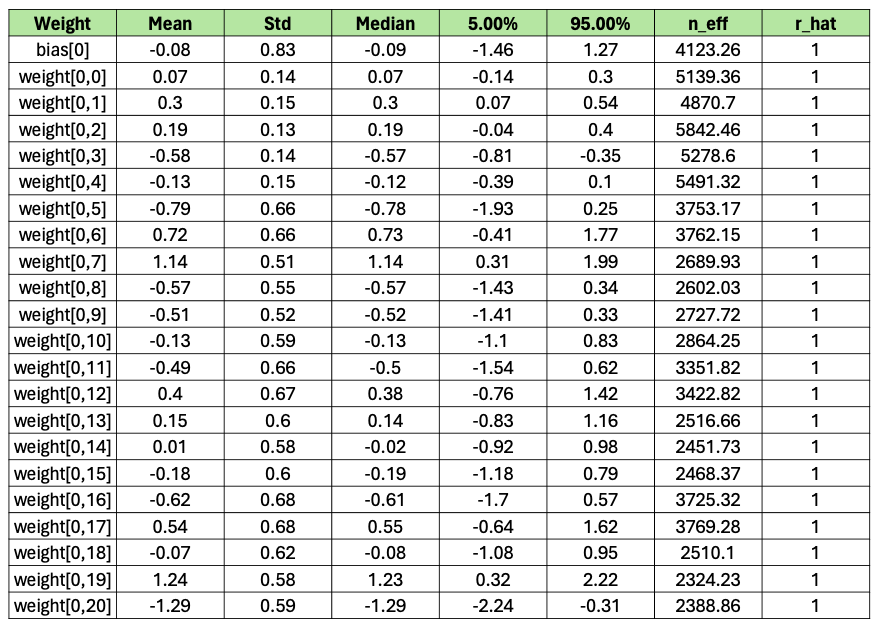
Applying the .summary() method to the class returned from the function above will print some summary statistics of the sampling. One of the columns printed is r_hat. This is the Gelman-Rubin statistic which assesses how well different chains have converged to the same posterior probability distribution after sampling the parameter space for each feature. A value of 1 for the Gelman-Rubin statistic is considered perfect convergence and generally, any value below 1.1 is considered so. A value greater than 1.2 indicates there is little convergence. I ran inference with four chains and 1000 samples, my output looks like this:
Sampling Summary
The first five columns provide descriptive statistics on the samples generated for each parameter. The r_hat values for all features indicate MCMC converged, meaning it is producing consistent estimations for each feature. The method also produces a metric ‘n_eff’, meaning an effective sample size. A large effective sample size relative to the number of samples taken is a strong sign that we have enough independent samples for reliable statistical inference, and that the samples are informative. The values of n_eff and r_hat here suggest strong model convergence and reliable results.
Plots can be generated to visualise the values sampled for each feature. Taking the first column of the matrix of weights we sampled as an example (corresponding to the first feature in the input data), generates the trace and probability density function below.
Trace and Kernel Density Plot — Image by Author
These plots help visualise uncertainty and convergence in the model. By calling the .get_samples() method and passing in the parameter group_by_chain = True, we can also evaluate the variety in sampling between chains. The plot below regenerates the plot above but groups the samples by the chain from which they were collected.
The subplot on the right demonstrates the model is consistently converging towards the same posterior distribution of the parameter value.
Generating Predictions
The prediction of the model is calculated by passing every set of samples drawn for the latent variables into the structure of the model. 4000 samples were collected, so we can generate 4000 predictions per example. The function below generates the class prediction for each example scored, a matrix of 4000 predictions per example and a tensor containing the mean prediction over 4000 samples per example scored.
The trace and kernel density plots of predictions for each example can be generated, to visualise the uncertainty of the predictions. The plots below illustrate the distribution of probabilities the model has produced for a random example in the test data set.
Trace and Distribution Plot of Model Predictions — Image by Author
Over the 4000 samples, the model consistently predicts the example belongs to the positive class (does have heart disease).
Model Evaluation
The code below contains a function which produces some evaluation metrics from the Sckit-learn metrics module.
The class_prediction and mean_prediction variables returned from the create_predictions function can be passed into this function to generate a dictionary of metrics to evaluate the performance of the model for the training and test datasets. The table below summarises this information for test and training data. By nature of sampling methods, these results will vary for each independent run of the MCMC algorithm. It should be noted that accuracy should not be used as a robust measure of model performance when working with unbalanced datasets. When working with unbalanced datasets, using metrics such as the F1 score is more appropriate. Approximately 55% of the examples in the dataset belonged to the positive class, so the imbalance is small.
Classification Evaluation Metrics — Image by Author
Precision tells us how many times the model predicted a patient had heart disease when they did. Recall tells us what proportion of patients who had heart disease were correctly predicted by the model. The importance of each of these metrics varies by the use case. In the medical industry, recall performance would be important as you would not want a situation where the model predicted a patient did not have heart disease when they did. In this model, the reduction in recall performance between the training and test data would be a concern. However, these metrics were generated using a standard cut-off of 0.5. The model’s threshold — the cut-off for classifying the positive and negative class — can be changed to improve recall. By reducing the threshold recall performance will improve, as fewer actual heart disease cases will be incorrectly identified. However, this will degrade the precision of the model, as more positive predictions will be false. The threshold of classification models is a method to manipulate the trade-off between these two metrics.
The AUC -ROC score for the training and test datasets is encouraging. As a general rule of thumb, a score above 0.9 indicates strong performance, which is true for both the training and test datasets. The graph below plots the AUC-ROC curve for both datasets.
Summary
This article aimed to provide a framework for solving binary classification problems using Bayesian methods, which I hope you have found useful. The model performs well across a range of evaluation metrics. However, model improvements are possible with a greater focus on feature engineering and selection.
In my previous article, I discussed Bayesian thinking in more depth. If you are interested, I have provided the link below. I have also provided a link to another article, which provides a good introduction to logistic regression modelling.
We use cookies on our website to give you the most relevant experience by remembering your preferences and repeat visits. By clicking “Accept”, you consent to the use of ALL the cookies.
This website uses cookies to improve your experience while you navigate through the website. Out of these, the cookies that are categorized as necessary are stored on your browser as they are essential for the working of basic functionalities of the website. We also use third-party cookies that help us analyze and understand how you use this website. These cookies will be stored in your browser only with your consent. You also have the option to opt-out of these cookies. But opting out of some of these cookies may affect your browsing experience.
Necessary cookies are absolutely essential for the website to function properly. These cookies ensure basic functionalities and security features of the website, anonymously.
Cookie
Duration
Description
cookielawinfo-checkbox-analytics
11 months
This cookie is set by GDPR Cookie Consent plugin. The cookie is used to store the user consent for the cookies in the category "Analytics".
cookielawinfo-checkbox-functional
11 months
The cookie is set by GDPR cookie consent to record the user consent for the cookies in the category "Functional".
cookielawinfo-checkbox-necessary
11 months
This cookie is set by GDPR Cookie Consent plugin. The cookies is used to store the user consent for the cookies in the category "Necessary".
cookielawinfo-checkbox-others
11 months
This cookie is set by GDPR Cookie Consent plugin. The cookie is used to store the user consent for the cookies in the category "Other.
cookielawinfo-checkbox-performance
11 months
This cookie is set by GDPR Cookie Consent plugin. The cookie is used to store the user consent for the cookies in the category "Performance".
viewed_cookie_policy
11 months
The cookie is set by the GDPR Cookie Consent plugin and is used to store whether or not user has consented to the use of cookies. It does not store any personal data.
Functional cookies help to perform certain functionalities like sharing the content of the website on social media platforms, collect feedbacks, and other third-party features.
Performance cookies are used to understand and analyze the key performance indexes of the website which helps in delivering a better user experience for the visitors.
Analytical cookies are used to understand how visitors interact with the website. These cookies help provide information on metrics the number of visitors, bounce rate, traffic source, etc.
Advertisement cookies are used to provide visitors with relevant ads and marketing campaigns. These cookies track visitors across websites and collect information to provide customized ads.