Month: February 2024

How to Forecast Time Series Data Using any Supervised Learning Model

Featurizing time series data into a standard tabular format for classical ML models and improving accuracy using AutoML

This article delves into enhancing the process of forecasting daily energy consumption levels by transforming a time series dataset into a tabular format using open-source libraries. We explore the application of a popular multiclass classification model and leverage AutoML with Cleanlab Studio to significantly boost our out-of-sample accuracy.

The key takeaway from this article is that we can utilize more general methods to model a time series dataset by converting it to a tabular structure, and even find improvements in trying to predict this time series data.

Take a Snapshot

At a high level we will:

• Establish a baseline accuracy by fitting a Prophet forecasting model on our time series data
• Convert our time series data into a tabular format by using open-source featurization libraries and then will show that can outperform our Prophet model with a standard multiclass classification (Gradient Boosting) approach by a 67% reduction in prediction error (increase by 38% raw percentage points in out-of-sample accuracy).
• Use an AutoML solution for multiclass classification resulted in a 42% reduction in prediction error (increase by 8% in raw percentage points in out-of-sample accuracy) compared to our Gradient Boosting model and resulted in a 81% reduction in prediction error (increase by 46% in raw percentage points in out-of-sample accuracy) compared to our Prophet forecasting model.

To run the code demonstrated in this article, here’s the full notebook.

Examine the Data

You can download the dataset here.

The data represents PJM hourly energy consumption (in megawatts) on an hourly basis. PJM Interconnection LLC (PJM) is a regional transmission organization (RTO) in the United States. It is part of the Eastern Interconnection grid operating an electric transmission system serving many states.

Let’s take a look at our dataset. The data includes one datetime column (object type), and the Megawatt Energy Consumption (float64) type) column we are trying to forecast as a discrete variable (corresponding to the quartile of hourly energy consumption levels). Our aim is to train a time series forecasting model to be able to forecast the tomorrow’s daily energy consumption level falling into 1 of 4 levels: low , below average , above average or high (these levels were determined based on quartiles of the overall daily consumption distribution). We first demonstrate how to apply time-series forecasting methods like Prophet to this problem, but these are restricted to certain types of ML models suitable for time-series data. Next we demonstrate how to reframe this problem into a standard multiclass classification problem that we can apply any machine learning model to, and show how we can obtain superior forecasts by using powerful supervised ML.

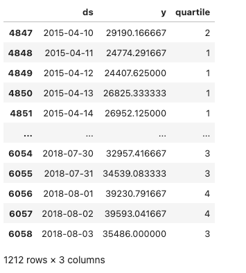
We first convert this data into a average energy consumption at a daily level and rename the columns to the format that the Prophet forecasting model expects. These real-valued daily energy consumption levels are converted into quartiles, which is the value we are trying to predict. Our training data is shown below along with the quartile each daily energy consumption level falls into. The quartiles are computed using training data to prevent data leakage.

We then show the test data below, which is the data we are evaluating our forecasting results against.

We then show the test data below, which is the data we are evaluating our forecasting results against.

Train and Evaluate Prophet Forecasting Model

As seen in the images above, we will use a date cutoff of 2015-04-09 to end the range of our training data and start our test data at 2015-04-10 . We compute quartile thresholds of our daily energy consumption using ONLY training data. This avoids data leakage – using out-of-sample data that is available only in the future.

Next, we will forecast the daily PJME energy consumption level (in MW) for the duration of our test data and represent the forecasted values as a discrete variable. This variable represents which quartile the daily energy consumption level falls into, represented categorically as 1 (low), 2 (below average), 3 (above average), or 4 (high). For evaluation, we are going to use the accuracy_score function from scikit-learn to evaluate the performance of our models. Since we are formulating the problem this way, we are able to evaluate our model’s next-day forecasts (and compare future models) using classification accuracy.

import numpy as np
from prophet import Prophet
from sklearn.metrics import accuracy_score

# Initialize model and train it on training data
model = Prophet()
model.fit(train_df)

# Create a dataframe for future predictions covering the test period
future = model.make_future_dataframe(periods=len(test_df), freq='D')
forecast = model.predict(future)

# Categorize forecasted daily values into quartiles based on the thresholds
forecast['quartile'] = pd.cut(forecast['yhat'], bins = [-np.inf] + list(quartiles) + [np.inf], labels=[1, 2, 3, 4])

# Extract the forecasted quartiles for the test period
forecasted_quartiles = forecast.iloc[-len(test_df):]['quartile'].astype(int)

# Categorize actual daily values in the test set into quartiles
test_df['quartile'] = pd.cut(test_df['y'], bins=[-np.inf] + list(quartiles) + [np.inf], labels=[1, 2, 3, 4])
actual_test_quartiles = test_df['quartile'].astype(int)

# Calculate the evaluation metrics
accuracy = accuracy_score(actual_test_quartiles, forecasted_quartiles)

# Print the evaluation metrics
print(f'Accuracy: {accuracy:.4f}')
>>> 0.4249

The out-of-sample accuracy is quite poor at 43%. By modelling our time series this way, we limit ourselves to only use time series forecasting models (a limited subset of possible ML models). In the next section, we consider how we can more flexibly model this data by transforming the time-series into a standard tabular dataset via appropriate featurization. Once the time-series has been transformed into a standard tabular dataset, we’re able to employ any supervised ML model for forecasting this daily energy consumption data.

Convert time series data to tabular data through featurization

Now we convert the time series data into a tabular format and featurize the data using the open source libraries sktime, tsfresh, and tsfel. By employing libraries like these, we can extract a wide array of features that capture underlying patterns and characteristics of the time series data. This includes statistical, temporal, and possibly spectral features, which provide a comprehensive snapshot of the data’s behavior over time. By breaking down time series into individual features, it becomes easier to understand how different aspects of the data influence the target variable.

TSFreshFeatureExtractor is a feature extraction tool from the sktime library that leverages the capabilities of tsfresh to extract relevant features from time series data. tsfresh is designed to automatically calculate a vast number of time series characteristics, which can be highly beneficial for understanding complex temporal dynamics. For our use case, we make use of the minimal and essential set of features from our TSFreshFeatureExtractor to featurize our data.

tsfel, or Time Series Feature Extraction Library, offers a comprehensive suite of tools for extracting features from time series data. We make use of a predefined config that allows for a rich set of features (e.g., statistical, temporal, spectral) to be constructed from the energy consumption time series data, capturing a wide range of characteristics that might be relevant for our classification task.

import tsfel
from sktime.transformations.panel.tsfresh import TSFreshFeatureExtractor

# Define tsfresh feature extractor
tsfresh_trafo = TSFreshFeatureExtractor(default_fc_parameters="minimal")

# Transform the training data using the feature extractor
X_train_transformed = tsfresh_trafo.fit_transform(X_train)

# Transform the test data using the same feature extractor
X_test_transformed = tsfresh_trafo.transform(X_test)

# Retrieves a pre-defined feature configuration file to extract all available features
cfg = tsfel.get_features_by_domain()

# Function to compute tsfel features per day
def compute_features(group):
    # TSFEL expects a DataFrame with the data in columns, so we transpose the input group
    features = tsfel.time_series_features_extractor(cfg, group, fs=1, verbose=0)
    return features


# Group by the 'day' level of the index and apply the feature computation
train_features_per_day = X_train.groupby(level='Date').apply(compute_features).reset_index(drop=True)
test_features_per_day = X_test.groupby(level='Date').apply(compute_features).reset_index(drop=True)

# Combine each featurization into a set of combined features for our train/test data
train_combined_df = pd.concat([X_train_transformed, train_features_per_day], axis=1)
test_combined_df = pd.concat([X_test_transformed, test_features_per_day], axis=1)

Next, we clean our dataset by removing features that showed a high correlation (above 0.8) with our target variable — average daily energy consumption levels — and those with null correlations. High correlation features can lead to overfitting, where the model performs well on training data but poorly on unseen data. Null-correlated features, on the other hand, provide no value as they lack a definable relationship with the target.

By excluding these features, we aim to improve model generalizability and ensure that our predictions are based on a balanced and meaningful set of data inputs.

# Filter out features that are highly correlated with our target variable
column_of_interest = "PJME_MW__mean"
train_corr_matrix = train_combined_df.corr()
train_corr_with_interest = train_corr_matrix[column_of_interest]
null_corrs = pd.Series(train_corr_with_interest.isnull())
false_features = null_corrs[null_corrs].index.tolist()

columns_to_exclude = list(set(train_corr_with_interest[abs(train_corr_with_interest) > 0.8].index.tolist() + false_features))
columns_to_exclude.remove(column_of_interest)

# Filtered DataFrame excluding columns with high correlation to the column of interest
X_train_transformed = train_combined_df.drop(columns=columns_to_exclude)
X_test_transformed = test_combined_df.drop(columns=columns_to_exclude)

If we look at the first several rows of the training data now, this is a snapshot of what it looks like. We now have 73 features that were added from the time series featurization libraries we used. The label we are going to predict based on these features is the next day’s energy consumption level.

It’s important to note that we used a best practice of applying the featurization process separately for training and test data to avoid data leakage (and the held-out test data are our most recent observations).

Also, we compute our discrete quartile value (using the quartiles we originally defined) using the following code to obtain our train/test energy labels, which is what our y_labels are.

# Define a function to classify each value into a quartile
def classify_into_quartile(value):
    if value < quartiles[0]:
        return 1  
    elif value < quartiles[1]:
        return 2  
    elif value < quartiles[2]:
        return 3  
    else:
        return 4  

y_train = X_train_transformed["PJME_MW__mean"].rename("daily_energy_level")
X_train_transformed.drop("PJME_MW__mean", inplace=True, axis=1)

y_test = X_test_transformed["PJME_MW__mean"].rename("daily_energy_level")
X_test_transformed.drop("PJME_MW__mean", inplace=True, axis=1)

energy_levels_train = y_train.apply(classify_into_quartile)
energy_levels_test = y_test.apply(classify_into_quartile)

Train and Evaluate GradientBoostingClassifier Model on featurized tabular data

Using our featurized tabular dataset, we can apply any supervised ML model to predict future energy consumption levels. Here we’ll use a Gradient Boosting Classifier (GBC) model, the weapon of choice for most data scientists operating on tabular data.

Our GBC model is instantiated from the sklearn.ensemble module and configured with specific hyperparameters to optimize its performance and avoid overfitting.

from sklearn.ensemble import GradientBoostingClassifier

gbc = GradientBoostingClassifier(
    n_estimators=150,
    learning_rate=0.1,
    max_depth=4,
    min_samples_leaf=20,
    max_features='sqrt',
    subsample=0.8,
    random_state=42
)

gbc.fit(X_train_transformed, energy_levels_train)


y_pred_gbc = gbc.predict(X_test_transformed)
gbc_accuracy = accuracy_score(energy_levels_test, y_pred_gbc)
print(f'Accuracy: {gbc_accuracy:.4f}')
>>> 0.8075

The out-of-sample accuracy of 81% is considerably better than our prior Prophet model results.

Using AutoML to streamline things

Now that we’ve seen how to featurize the time-series problem and the benefits of applying powerful ML models like Gradient Boosting, a natural question emerges: Which supervised ML model should we apply? Of course, we could experiment with many models, tune their hyperparameters, and ensemble them together. An easier solution is to let AutoML handle all of this for us.

Here we’ll use a simple AutoML solution provided in Cleanlab Studio, which involves zero configuration. We just provide our tabular dataset, and the platform automatically trains many types of supervised ML models (including Gradient Boosting among others), tunes their hyperparameters, and determines which models are best to combine into a single predictor. Here’s all the code needed to train and deploy an AutoML supervised classifier:

from cleanlab_studio import Studio

studio = Studio()
studio.create_project(
    dataset_id=energy_forecasting_dataset,
    project_name="ENERGY-LEVEL-FORECASTING",
    modality="tabular",
    task_type="multi-class",
    model_type="regular",
    label_column="daily_energy_level",
)

model = studio.get_model(energy_forecasting_model)
y_pred_automl = model.predict(test_data, return_pred_proba=True)

Below we can see model evaluation estimates in the AutoML platform, showing all of the different types of ML models that were automatically fit and evaluated (including multiple Gradient Boosting models), as well as an ensemble predictor constructed by optimally combining their predictions.

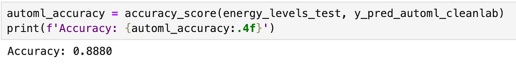
After running inference on our test data to obtain the next-day energy consumption level predictions, we see the test accuracy is 89%, a 8% raw percentage points improvement compared to our previous Gradient Boosting approach.

Conclusion

For our PJM daily energy consumption data, we found that transforming the data into a tabular format and featurizing it achieved a 67% reduction in prediction error (increase by 38% in raw percentage points in out-of-sample accuracy) compared to our baseline accuracy established with our Prophet forecasting model.

We also tried an easy AutoML approach for multiclass classification, which resulted in a 42% reduction in prediction error (increase by 8% in raw percentage points in out-of-sample accuracy) compared to our Gradient Boosting model and resulted in a 81% reduction in prediction error (increase by 46% in raw percentage points in out-of-sample accuracy) compared to our Prophet forecasting model.

By taking approaches like those illustrated above to model a time series dataset beyond the constrained approach of only considering forecasting methods, we can apply more general supervised ML techniques and achieve better results for certain types of forecasting problems.

Unless otherwise noted, all images are by the author.

How to Forecast Time Series Data using any Supervised Learning Model was originally published in Towards Data Science on Medium, where people are continuing the conversation by highlighting and responding to this story.

An astounding number of videos are available on the Web, covering a variety of content from everyday moments people share to historical moments to scientific observations, each of which contains a unique record of the world. The right tools could help researchers analyze these videos, transforming how we understand the world around us.

Videos offer dynamic visual content far more rich than static images, capturing movement, changes, and dynamic relationships between entities. Analyzing this complexity, along with the immense diversity of publicly available video data, demands models that go beyond traditional image understanding. Consequently, many of the approaches that best perform on video understanding still rely on specialized models tailor-made for particular tasks. Recently, there has been exciting progress in this area using video foundation models (ViFMs), such as VideoCLIP, InternVideo, VideoCoCa, and UMT). However, building a ViFM that handles the sheer diversity of video data remains a challenge.

With the goal of building a single model for general-purpose video understanding, we introduced “VideoPrism: A Foundational Visual Encoder for Video Understanding”. VideoPrism is a ViFM designed to handle a wide spectrum of video understanding tasks, including classification, localization, retrieval, captioning, and question answering (QA). We propose innovations in both the pre-training data as well as the modeling strategy. We pre-train VideoPrism on a massive and diverse dataset: 36 million high-quality video-text pairs and 582 million video clips with noisy or machine-generated parallel text. Our pre-training approach is designed for this hybrid data, to learn both from video-text pairs and the videos themselves. VideoPrism is incredibly easy to adapt to new video understanding challenges, and achieves state-of-the-art performance using a single frozen model.

Pre-training data

A powerful ViFM needs a very large collection of videos on which to train — similar to other foundation models (FMs), such as those for large language models (LLMs). Ideally, we would want the pre-training data to be a representative sample of all the videos in the world. While naturally most of these videos do not have perfect captions or descriptions, even imperfect text can provide useful information about the semantic content of the video.

To give our model the best possible starting point, we put together a massive pre-training corpus consisting of several public and private datasets, including YT-Temporal-180M, InternVid, VideoCC, WTS-70M, etc. This includes 36 million carefully selected videos with high-quality captions, along with an additional 582 million clips with varying levels of noisy text (like auto-generated transcripts). To our knowledge, this is the largest and most diverse video training corpus of its kind.

Statistics on the video-text pre-training data. The large variations of the CLIP similarity scores (the higher, the better) demonstrate the diverse caption quality of our pre-training data, which is a byproduct of the various ways used to harvest the text.

Two-stage training

The VideoPrism model architecture stems from the standard vision transformer (ViT) with a factorized design that sequentially encodes spatial and temporal information following ViViT. Our training approach leverages both the high-quality video-text data and the video data with noisy text mentioned above. To start, we use contrastive learning (an approach that minimizes the distance between positive video-text pairs while maximizing the distance between negative video-text pairs) to teach our model to match videos with their own text descriptions, including imperfect ones. This builds a foundation for matching semantic language content to visual content.

After video-text contrastive training, we leverage the collection of videos without text descriptions. Here, we build on the masked video modeling framework to predict masked patches in a video, with a few improvements. We train the model to predict both the video-level global embedding and token-wise embeddings from the first-stage model to effectively leverage the knowledge acquired in that stage. We then randomly shuffle the predicted tokens to prevent the model from learning shortcuts.

What is unique about VideoPrism’s setup is that we use two complementary pre-training signals: text descriptions and the visual content within a video. Text descriptions often focus on what things look like, while the video content provides information about movement and visual dynamics. This enables VideoPrism to excel in tasks that demand an understanding of both appearance and motion.

Results

We conducted extensive evaluation on VideoPrism across four broad categories of video understanding tasks, including video classification and localization, video-text retrieval, video captioning, question answering, and scientific video understanding. VideoPrism achieves state-of-the-art performance on 30 out of 33 video understanding benchmarks — all with minimal adaptation of a single, frozen model.

VideoPrism compared to the previous best-performing FMs.

Classification and localization

We evaluate VideoPrism on an existing large-scale video understanding benchmark (VideoGLUE) covering classification and localization tasks. We found that (1) VideoPrism outperforms all of the other state-of-the-art FMs, and (2) no other single model consistently came in second place. This tells us that VideoPrism has learned to effectively pack a variety of video signals into one encoder — from semantics at different granularities to appearance and motion cues — and it works well across a variety of video sources.

VideoPrism outperforms state-of-the-art approaches (including CLIP, VATT, InternVideo, and UMT) on the video understanding benchmark. In this plot, we show the absolute score differences compared with the previous best model to highlight the relative improvements of VideoPrism. On Charades, ActivityNet, AVA, and AVA-K, we use mean average precision (mAP) as the evaluation metric. On the other datasets, we report top-1 accuracy.

Combining with LLMs

We further explore combining VideoPrism with LLMs to unlock its ability to handle various video-language tasks. In particular, when paired with a text encoder (following LiT) or a language decoder (such as PaLM-2), VideoPrism can be utilized for video-text retrieval, video captioning, and video QA tasks. We compare the combined models on a broad and challenging set of vision-language benchmarks. VideoPrism sets the new state of the art on most benchmarks. From the visual results, we find that VideoPrism is capable of understanding complex motions and appearances in videos (e.g., the model can recognize the different colors of spinning objects on the window in the visual examples below). These results demonstrate that VideoPrism is strongly compatible with language models.

VideoPrism achieves competitive results compared with state-of-the-art approaches (including VideoCoCa, UMT and Flamingo) on multiple video-text retrieval (top) and video captioning and video QA (bottom) benchmarks. We also show the absolute score differences compared with the previous best model to highlight the relative improvements of VideoPrism. We report the Recall@1 on MASRVTT, VATEX, and ActivityNet, CIDEr score on MSRVTT-Cap, VATEX-Cap, and YouCook2, top-1 accuracy on MSRVTT-QA and MSVD-QA, and WUPS index on NExT-QA.

Scientific applications

Finally, we tested VideoPrism on datasets used by scientists across domains, including fields such as ethology, behavioral neuroscience, and ecology. These datasets typically require domain expertise to annotate, for which we leverage existing scientific datasets open-sourced by the community including Fly vs. Fly, CalMS21, ChimpACT, and KABR. VideoPrism not only performs exceptionally well, but actually surpasses models designed specifically for those tasks. This suggests tools like VideoPrism have the potential to transform how scientists analyze video data across different fields.

VideoPrism outperforms the domain experts on various scientific benchmarks. We show the absolute score differences to highlight the relative improvements of VideoPrism. We report mean average precision (mAP) for all datasets, except for KABR which uses class-averaged top-1 accuracy.

Conclusion

With VideoPrism, we introduce a powerful and versatile video encoder that sets a new standard for general-purpose video understanding. Our emphasis on both building a massive and varied pre-training dataset and innovative modeling techniques has been validated through our extensive evaluations. Not only does VideoPrism consistently outperform strong baselines, but its unique ability to generalize positions it well for tackling an array of real-world applications. Because of its potential broad use, we are committed to continuing further responsible research in this space, guided by our AI Principles. We hope VideoPrism paves the way for future breakthroughs at the intersection of AI and video analysis, helping to realize the potential of ViFMs across domains such as scientific discovery, education, and healthcare.

Acknowledgements

This blog post is made on behalf of all the VideoPrism authors: Long Zhao, Nitesh B. Gundavarapu, Liangzhe Yuan, Hao Zhou, Shen Yan, Jennifer J. Sun, Luke Friedman, Rui Qian, Tobias Weyand, Yue Zhao, Rachel Hornung, Florian Schroff, Ming-Hsuan Yang, David A. Ross, Huisheng Wang, Hartwig Adam, Mikhail Sirotenko, Ting Liu, and Boqing Gong. We sincerely thank David Hendon for their product management efforts, and Alex Siegman, Ramya Ganeshan, and Victor Gomes for their program and resource management efforts. We also thank Hassan Akbari, Sherry Ben, Yoni Ben-Meshulam, Chun-Te Chu, Sam Clearwater, Yin Cui, Ilya Figotin, Anja Hauth, Sergey Ioffe, Xuhui Jia, Yeqing Li, Lu Jiang, Zu Kim, Dan Kondratyuk, Bill Mark, Arsha Nagrani, Caroline Pantofaru, Sushant Prakash, Cordelia Schmid, Bryan Seybold, Mojtaba Seyedhosseini, Amanda Sadler, Rif A. Saurous, Rachel Stigler, Paul Voigtlaender, Pingmei Xu, Chaochao Yan, Xuan Yang, and Yukun Zhu for the discussions, support, and feedback that greatly contributed to this work. We are grateful to Jay Yagnik, Rahul Sukthankar, and Tomas Izo for their enthusiastic support for this project. Lastly, we thank Tom Small, Jennifer J. Sun, Hao Zhou, Nitesh B. Gundavarapu, Luke Friedman, and Mikhail Sirotenko for the tremendous help with making this blog post.